
Measuring the firm-level impact of the Canadian Technology Accelerator program
Colin Scarffe
January 2024
Key points
- Participating in the Canadian Technology Accelerator (CTA) program resulted in 27% greater revenues one year after completing the program compared to similar firms which did not participate in the program. Comparable positive results were observed for assets, payroll, expenditures, and Scientific Research and Experimental Development (SRED) expenditures.
- With these results we can estimate that on average, the typical CTA client firm sees a $1.3 million increase in revenue one year after completing the CTA program. This estimate overlooks potential variations in treatment effects based on firm size and is evaluated at the mean revenue of $3.5 million.
- The effects of the program increase and remains statistically significant as more time elapses from program completion. The results are robust across a variety of estimation techniques and econometric specifications.
- CTA program participants experienced faster growth compared to non-participating firms in the same industry over the same period. Growth, as measured by revenue, assets, payroll, expenditures, SRED expenditures, and investment in machinery and equipment, consistently demonstrated faster rates for CTA firms, both in the year following program completion and for at least five years thereafter.
Non-technical Summary
The Canadian Technology Accelerator (CTA) program, administered by Global Affairs Canada since 2013, was introduced to facilitate the international expansion of high-potential Canadian Small and Medium Enterprises (SMEs). Previous reports, including the "Results and Outcomes Report 2019-2020" and the program evaluation for the Federal Government budget renewal in 2023, have highlighted positive outcomes such as increased revenue, job creation, and capital raised for CTA firms. This study starts by finding similar correlations. Firms that participated in the CTA experienced accelerated growth in revenue, assets, payroll, expenditures, Scientific Research and Experimental Development (SRED) expenditures, and investment in machinery and equipment.
However, the previous studies and the initial correlations in this report fail to account for the potential selection bias of considering what subset of firms choose to participate in the CTA program. Consequently, distinguishing between the active contribution of the CTA to firm success and program administrators selecting firms that were already poised for success remains unclear. This study aims to rectify this by tackling selection bias and providing an estimate of the causal effect of the CTA program.
Using an econometric technique known as matching, this study finds that firms that participated in the CTA program have better outcomes when compared with non-participating firms with otherwise similar characteristics. The goal of the matching strategy is to compare firms that are as similar as possible, thereby attributing differences in outcomes to their participation in the program. In the preferred specification, each CTA participant was matched to five non-participating firms in the year prior to participation in the program, in the same industry and possessing comparable age, revenue, assets, payroll, expenditures, SRED expenditure, and investment in machinery and equipment.
Using the matching strategy, this study finds that participating in the CTA program resulted in 27% greater revenues one year after completing the program compared to similar firms which did not participate in the program. With these results we can estimate that on average, the typical CTA client firm sees a $1.3 million increase in revenue one year after completing the CTA program. This estimate is evaluated at the average revenue of a CTA firm of $3.5 million. Similar positive effects were observed for assets, payroll, expenditures, and SRED expenditures, but not for investment in machinery and equipment. The effects were even stronger five years after participating in the program.
An additional finding is that relative to the period before CTA participation, firms that have completed the CTA program exhibit elevated levels of revenue, assets, payroll, expenditures, and SRED expenditures. However, when evaluating the growth of these variables, the program's impact is either statistically indistinguishable from zero, or in some cases, there is evidence suggesting a slowdown in growth. While this may appear as a negative outcome, it could signify that CTA firms are predominantly fast-growing entities, and their growth naturally decelerates over time. Further investigation is required to ascertain whether the CTA contributes to higher firm growth compared to a scenario without the program.
1. Introduction
The Canadian Technology Accelerator (CTA) program was introduced by Global Affairs Canada in 2013 to facilitate the international expansion of high-potential Canadian Small and Medium Enterprises (SMEs). Operating from Canada's various missions abroad, the program spans three to eight months, bringing together 6 to 12 companies at similar stages of development within the same sector. The CTA's objective is to foster the growth of Canadian SMEs in technology-focused sectors, providing tailored services such as business development support, strategic guidance, assistance in engaging service providers, and connections to potential clients, partners, and investors. The program primarily collaborates with companies in cleantech, digital technologies, and life sciences.
The CTA program has demonstrated success across various metrics collected from participating firms. According to the “Results and Outcomes Report 2019-2020”, CTA firms have cumulatively generated $239 million in new revenue, created over 2,500 new jobs, have raised close to $650 million in new capital, and have established 45 new strategic partnerships.
As part of its periodic review, the program underwent evaluation during the Federal Government budget renewal in 2023. The evaluation found many encouraging examples of short-, medium-, and long-term outcomes and economic impacts. Notable outcomes include CTA firms increasing their client base and networks, expanding operations in a foreign market, increasing revenues, creating jobs at home and abroad, and increasing capital investment.
The positive indicators mentioned above suggest that firms participating in the CTA program are successful thereafter. However, these statistics do not offer insight into the extent to which the program contributes to this success. The CTA focuses on high-potential SMEs, implying that these companies might have been successful independently of their involvement in the program. Consequently, a pertinent question arises: does the CTA actively contribute to firms' enhanced success, or are the program administrators adept at selecting firms already poised for success?
This analysis attempts to estimate the causal effect of the CTA program on Canadian firms while addressing the selection bias through econometric techniques. There are three econometric techniques employed in this study including: conditioning on covariates; using various matching estimators and a non-parametric conditional difference-in-difference strategy à la Heckmen et al. (1997); and implementing firm fixed-effects estimation. This paper takes advantage of firm-level data from the Statistics Canada National Accounts Longitudinal Microdata File (NALMF) between 2013 and 2019.
This study finds that the CTA program causes participating firms to gain higher revenue, increased assets, a larger payroll, more expenditures, and more Scientific Research and Experimental Development (SRED) expenditures. One-year after completing the program, firms have 27% higher revenue compared to firms in the same industry and year, with similar characteristics. Disregarding potential heterogeneous treatment effects based on firm size, the average treatment effect on the treated, evaluated at the mean revenue of $3.5 million, implies an average increase of $1.3 million in revenue per firm one year after completing the CTA program.
The findings remain consistent across various estimators; furthermore, they demonstrate a strengthening trend over time—specifically, the effects are more pronounced three and five years after the firm exits the CTA program compared to the year immediately after completion. While one of the programs stated goals is to help firms become more international, there is insufficient data to test these angles.
Firm fixed-effects confirm that, in level, the results are not confined to comparing across firms. Comparing temporally within the firms, the results from the firm fixed-effects indicate strong positive effects in log-level once the firms have completed the CTA program. However, using firm fixed-effects and the difference in log-level suggests a potential deceleration in the growth of these firms after the program. The deceleration in growth may not be inherently negative as existing literature suggest that most fast-growing firms tend to experience a natural slowdown over time as they age and get larger. Regrettably, the sample size is insufficient to establish a counterfactual for firm growth.
The paper is organized as follows: Section two provides straightforward summary statistics, and a simple growth comparison of CTA firms with non-CTA firms. Section three provides the econometric methodology for the regressions and the matching estimators. Section four contains the econometric results from the matching estimators. Section five contains the fixed-effects results. Finally, section six concludes the paper.
2. Data, summary statistics, and a simple growth comparison
The primary data source for this paper is the Statistics Canada National Accounts Longitudinal Microdata File (NALMF), accessed through the Statistics Canada virtual data lab. The NALMF dataset is constructed using annual cross-section files, with firms identified over years through a unique ID number. This ID number ensures the longitudinal nature of the dataset, allowing for the tracking of individual firms over time (Rivard, 2020). Business register numbers of firms that participated in the CTA program were provided by Global Affairs Canada, and Statistics Canada successfully linked these firms to the unique ID in the NALMF dataset, with a linkage rate of 92%, enabling the analysis of CTA firms using the NALMF data.
The CTA program was initiated in 2013 and remains active. However, for the purpose of this report, data analysis covers the period from 2013 to 2020. Due to potential distortions caused by the pandemic in 2020, the report concludes with the data available up to 2019. The dataset includes information on over 400 firms, with annual participation ranging from 35 to 80, as seen in table 1.
Table 1: Year of CTA participating firmsFootnote 1
| Year | Number of participating firms | Proportion |
|---|---|---|
| 2013 | 55 | 13% |
| 2014 | 65 | 16% |
| 2015 | 65 | 16% |
| 2016 | 60 | 14% |
| 2017 | 35 | 8% |
| 2018 | 80 | 19% |
| 2019 | 55 | 13% |
| Total | 415 | 100% |
Predominantly, the clients are in technology-related industries. 125 are in NAICS 5415 (Computer systems design and related services), 70 are in NAICS 5417 (Scientific research and development services), 30 are in NAICS 5112 (Software publishers), and 20 are in 5416 (Management, scientific, and technical consulting services). The other industries with CTA clients only have a few firms per industry.
The variables of interest are chosen based off stated program goals, as well as the stated successes of the program such as increased revenue, assets, and jobs (which is measured through payroll in this study). Table 2 provides some measures of central tendency for the CTA participating firms in the year they participated in the CTA.
Table 2: Measures of central tendency on key variables for CTA firms during their CTA year.
| Revenue | Assets | Payroll | SRED expenditures | Investment in intangible | Exports | |
|---|---|---|---|---|---|---|
| Mean | $3,528,768 | $12,300,000 | $3,380,101 | $587,334 | $146,442 | $2,056,219 |
| Standard Deviation | 23,600,000 | 190,000,000 | 33,700,000 | 1,771,854 | 617,512 | 4,624,080 |
| Count | 410 | 410 | 375 | 305 | 70 | 70 |
On average, firms engaged in the CTA program report revenues of approximately $3.5 million in the year of program participation, accompanied by assets exceeding $12 million. A noteworthy feature across all variables is the considerable standard deviation, indicating substantial variability in the size of firms within the program, with some significantly smaller and others considerably larger than the average revenue of $3.5 million. In addition to the aforementioned variables, another noteworthy variable is profit. While technically 415 firms have reported a profit in the NALMF dataset, 365 of those observations are zero. Consequently, due to the prevalence of zero-profit observations, profit is largely ignored in this study.
Before delving into econometrics, a basic growth comparison is employed to assess whether firms exhibit positive outcomes in comparison to other firms upon completing the CTA program. While this comparison does not provide conclusive evidence of a causal relationship, which is the primary aim of the econometric analysis, it offers suggestive insights into potential effects of the CTA program on different outcomes. The primary advantage of these summary statistics lies in their accessibility and ease of interpretation compared to more complex econometric methods.
For the growth comparison, the 10 variables listed in table 2 were compared in the year immediately following the completion of the CTA with the year before the firm entered the CTA. For instance, if a firm went through the CTA program in 2013, the comparison involved the firm’s revenue in 2014 against its revenue in 2012. However, solely examining firm growth presents a challenge as it is unclear what would have occurred in absence of the CTA program. In addition, economic conditions significantly influence firm performance, with prosperous years generally benefiting most firms and recessions impacting them adversely. Thus, these statistics are improved when they are compared to firms that did not participate in the CTA program. If the firms that participated in the CTA have faster growth than their non-participating counterparts, this initial evidence suggests a positive impact of the CTA on firm growth.
Making a comparison between companies that participated in the CTA program and any random firm in the broader economy lacks practical utility. Notably, the CTA primarily caters to technology firms, so comparing a CTA firm with a company operating in a vastly distinct industry is impractical in the context. To establish a more meaningful comparison group, the firms in the comparison (or control) group must belong to the same industry (at the four-digit NAICS level) and cover the same years. Furthermore, the average age of the firm that participated in the CTA program was 5.9 years old, with a standard deviation of 4.85. Due to the relatively youthful nature of these firms, only firms under 11 years old were included in the control group. Each outcome was put into natural log in order to give it the interpretation of approximate percentage change, rather than change in level.
Additionally, the analysis extends its focus to outcomes beyond one year after the program. Evaluating the success of the program may place greater significance on firms demonstrating improved outcomes five years after program completion rather than immediately afterward. However, given the relatively recent inception of the CTA program, table 1 shows that there are only 7 years of usable data. Consequently, as the number of years post-program increases, the sample size diminishes rapidly. For some variables, the sample size is already small for a comparison one-year after the completion of the CTA.
Lastly, the average change in the variable in the treatment group will always be different than the average change in the variable in the control group—but it does not mean that the differences are meaningful. To determine whether the differences between the two groups are meaningful, standard errors were constructed to determine statistical significance. For each industry-year combination, the simple average of firm outcomes was computed and then differenced from the control group. This was than aggregated using a simple average (where the weight was the number of firms in each industry-year combination that participated in the CTA) to form the average difference in outcomes. The standard errors were estimated in two ways, the first was performing a bootstrapping procedure of the simple of industry-year difference in outcomes regardless of how many CTA firms were in each industry-year combination. The second was to do a weighted bootstrapping procedure where each industry-year outcomes were replicated to match the number of CTA firms that made up that observation. The statistical significance was not, in general, affected by which bootstrapping procedure was used. The results of the summary statistics are found in table 3, with statistically significant estimates in bold.
Table 3: A growth comparison for firms in the years following the CTA program compared to the year before the CTA program, measured against non-CTA firms
| Unweighted N | Unweighted Mean | Unweighted T-statistic | Weighted N | Weighted Mean | Weighted T-statistic | |
|---|---|---|---|---|---|---|
| ln_revenue_1 (1 year after CTA) | 134 | 0.84 | 9.02 | 323 | 0.81 | 17.98 |
| ln_revenue_2 (2 years after CTA) | 111 | 0.79 | 6.37 | 261 | 0.84 | 13.88 |
| ln_revenue_3 | 79 | 0.90 | 4.69 | 191 | 1.14 | 12.41 |
| ln_revenue_4 | 61 | 1.18 | 4.18 | 155 | 1.25 | 10.13 |
| ln_revenue_5 | 45 | 1.45 | 3.57 | 108 | 1.35 | 7.62 |
| ln_assets_1 | 137 | 0.60 | 6.02 | 331 | 0.58 | 12.33 |
| ln_assets_2 | 114 | 0.61 | 5.24 | 266 | 0.62 | 10.35 |
| ln_assets_3 | 82 | 1.00 | 5.91 | 199 | 0.85 | 10.62 |
| ln_assets_4 | 63 | 1.09 | 4.93 | 160 | 0.83 | 7.76 |
| ln_assets_5 | 47 | 1.30 | 4.75 | 113 | 1.02 | 7.7 |
| ln_payroll_1 | 127 | 0.47 | 6.31 | 298 | 0.44 | 10.95 |
| ln_payroll_2 | 104 | 0.56 | 6.47 | 237 | 0.56 | 11.96 |
| ln_payroll_3 | 77 | 0.73 | 5.39 | 175 | 0.73 | 10.46 |
| ln_payroll_4 | 60 | 0.83 | 5.11 | 142 | 0.71 | 8.47 |
| ln_payroll_5 | 46 | 0.82 | 3.36 | 96 | 0.8 | 6.37 |
| ln_expenses_1 | 136 | 0.65 | 11.51 | 331 | 0.67 | 21.94 |
| ln_expenses_2 | 113 | 0.64 | 6.86 | 268 | 0.69 | 13.72 |
| ln_expenses_3 | 81 | 0.76 | 6.34 | 197 | 0.9 | 15.01 |
| ln_expenses_4 | 62 | 0.99 | 6.00 | 159 | 1.02 | 13.39 |
| ln_expenses_5 | 46 | 1.00 | 4.03 | 112 | 1.03 | 8.92 |
| ln_sred_exp_1 | 97 | 0.33 | 3.12 | 220 | 0.25 | 4.72 |
| ln_sred_exp_2 | 77 | 0.41 | 3.99 | 165 | 0.35 | 5.73 |
| ln_sred_exp_3 | 55 | 0.27 | 2.06 | 125 | 0.36 | 4.76 |
| ln_sred_exp_4 | 46 | 0.24 | 1.53 | 107 | 0.38 | 4.77 |
| ln_sred_exp_5 | 31 | 0.28 | 1.51 | 70 | 0.35 | 3.7 |
| ln_investment ME_1 | 96 | 0.22 | 1.17 | 204 | 0.26 | 2.58 |
| ln_investment ME_2 | 84 | 0.35 | 1.86 | 162 | 0.38 | 3.13 |
| ln_investment ME_3 | 62 | 0.54 | 2.38 | 122 | 0.58 | 4.36 |
| ln_investment ME_4 | 46 | 0.55 | 2.03 | 94 | 0.56 | 3.24 |
| ln_investment ME_5 | 34 | 1.01 | 2.86 | 71 | 0.83 | 4.14 |
| ln_intangible Assets_1 | 45 | 0.21 | 1.75 | 62 | 0.18 | 1.95 |
| ln_investment BLDG_1 | 24 | 0.18 | 0.51 | 29 | 0.11 | 0.35 |
| ln_investment INTANGIBLE_1 | 14 | 0.67 | 3.40 | 14 | 0.67 | 3.51 |
| ln_exports_1 | 36 | 0.64 | 1.83 | 44 | 0.65 | 2.21 |
| ln_profit_1 | 20 | 1.21 | 2.37 | 22 | 1.08 | 2.17 |
To give an interpretation of first row of the table, there were 323 firms (weighted N) which participated in the CTA, with available revenue data one year before and one year after their CTA engagement. These firms represent 134 industry-year combinations (unweighted N). The unweighted mean indicates that CTA-participating firms experienced higher revenue growth than their non-CTA counterparts. Specifically, the growth from one year prior to the CTA to one year after the CTA was 0.84 natural-log points higher than firms who did not participate in the CTA, in the same industry, over the same years. Using a weighted average, the growth was 0.81 natural-log points, equivalent to approximately 130 percentage points.Footnote 2 In essence, firms in the CTA program had their revenue grow roughly 130 percentage points greater, on average, compared to non-CTA firms in the same industry and year.
The growth comparison presents a clear picture; firms that participated in the CTA have better outcomes than firms that did not participate in the CTA. CTA-participating firms exhibit higher growth across various dimensions, including revenue, assets, payroll, expenditure, SRED expenditure, and investment in machinery and equipment, when compared with their non-CTA counterparts. The sample size is too small to draw any definitive conclusions on the stock of intangible assets, investment in buildings, investment in intangible assets, export growth, or profit growth; but in the limited sample the results are also positive, albeit often not statistically different from zero.
For revenue, assets, payroll, expenditures, and investment in machinery and equipment, the effect increases as time extends. Five years after firms have completed the CTA program, the disparities in these outcomes are more pronounced when contrasted with non-CTA firms, compared to the year immediately after. This implies that firms sustain their success over time, indicating that the CTA does not merely offer a temporary boost but contributes to enduring positive effects.
The growth comparison aims to offer suggestive and easily comprehensible insights by comparing average outcomes with non-CTA firms in the same industry, the same year, and of similar age. While these insights are valuable, the growth comparison still exhibits selection bias. The following section employs econometrics to refine this comparison and attempt to eliminate the selection bias.
3. Econometric Methods
This study aims to assess the causal impact of the CTA program, with a specific focus on estimating either the average treatment effect (ATE) or the average treatment effect on the treated (ATT). The ATE pertains to the overall impact that the CTA program would have on the average firm within the sample, while the ATT specifically measures the average impact of the CTA program on firms that actively participated in it (i.e., the treated firms). A more thorough description of the ATE and ATT can be found in Van Biesebroeck, Yu, & Chen (2015).
If it were feasible to observe the outcomes of firms in both treated and untreated states, estimating the causal effect would be straightforward. Regrettably, the concurrent observation of the same firm under both treated and untreated conditions is unattainable. As a substitute, econometric methods are employed to estimate the treatment effect. The basic Ordinary Least Squares (OLS) regression is represented by Equation (1):

Text version
The outcome of interest, y, of firm i, in industry j, at time t, is equal to a constant, c, plus the correlation coefficient, beta 1, multiplied by treatment status, of firm i, in industry j, at time t, plus an error term, epsilon, of firm i, in industry j, at time t.
In equation (1), yi,j,t denotes the outcome for firm i, in industry j, at time t, c is a constant term, β1 represents the coefficient associated with the treatment indicator Ti,j,t, and εi,j,t signifies the error term. The treatment status is a dummy variable, which takes the value of zero when the firm has not undergone treatment (either prior to entry into the CTA program or if the firm has never been in the program) and equals one after the firms has completed the program.
The most pressing endogeneity concern with the simple OLS regression is the potential for selection bias into the CTA program. The concern arises from the possibility that the firms participating in the CTA program differ from those that do not participate in the program. In essence, it is plausible that firms in the CTA program may exhibit better outcomes than those not in the program, irrespective of actual program participation. By observing the differences in the outcome, the OLS estimate of the treatment effect is a combination of the true treatment effect, plus the selection bias. In order to achieve a non-biased causal estimate, the model needs to satisfy the condition-independence assumption which states that there is no dependence between being treated and potential outcomes.Footnote 3 Stated differently, selection bias is the concern that there is a correlation between firm outcome and selection into the program.
Randomly assigning which firms participate in the CTA program would alleviate the selection bias, as randomization inherently eliminates any correlation between firm outcome and selection into the program. However, firms have not been randomly assigned to the CTA program; rather, they have been chosen through a process involving self-selection and selection by the program administrators.
Instead of randomization, the econometrics in this paper will attempt to account for the differences between the treated firms and untreated firms. Two approaches are considered for accounting for these differences. Firstly, OLS regression is used to control for other variables by projecting the variable of interest into the span orthogonal to the other variables. Secondly, various matching estimators are employed to compare firms with similar characteristics. Both methods are valid causal strategies, provided that treatment status is as good as randomly assigned, conditional on covariates.Footnote 4
While various matching estimators are available and will be elaborated upon below, the critical factor lies in variable selection. The absence of covariates capable of accounting for the selection bias renders both OLS and matching strategies unsuitable for estimating the causal effect. In the context of matching strategies, the goal is to identify control observations closely resembling CTA firms prior to entering the CTA. Ideally, to satisfy the ignorability assumption, any variable that is correlated with both treatment status and outcome should be included.Footnote 5 Footnote 6 However, in the cases where the sample size is small, priority should be given to variable believed to be related to the outcome.Footnote 7 Footnote 8
The most important covariate included is the lag of the outcome variable. E.g. if the outcome of interest is revenue after the firm has completed the CTA, revenue prior to the firm entering the CTA is included. The rationale for including the outcome of interest at a lag can be justified in two ways. Firstly, the lagged-outcome acts in the context of a non-parametric conditional difference-in-difference estimator.Footnote 9 As articulated by Heckman et al., “From an economic standpoint [using the non-parametric conditional difference-in-difference estimator] is an attractive estimator because, unlike conventional matching estimators, it permits selection to be based on potential programme outcomes and allows for selection on unobservables. In particular, it is consistent with a Roy model of self selection applied to a panel setting”.Footnote 10
A second, less technical, perspective underscores the inclusion of the lagged variable by noting that when comparing the outcomes of two firms after treatment, their pre-treatment levels should be comparable. In this context, if revenue is being compared after participating in the CTA, the firms should have similar revenue levels prior to entering the CTA. In most circumstances, the main limitation of this technique lies in its dependence on panel data. However, this is not a constraint in this study, given the structure of the Statistics Canada longitudinal data.
In principle, when the outcome variable of interest changes, the corresponding variable included at a lag also changes. For instance, if the outcome variable is revenue, then lagged revenue is included; if the outcome variable is assets, then lagged assets are included. However, there is no restriction against incorporating all outcomes of interest, each at a lag, in every regression. This practice enhances the matches of the firms and hopefully further reduces potential selection bias. The downside of this approach is the reduction in sample size.
Additionally, other variables present in the summary statistics were included, namely, the year, industry (at the four-digit NAICS level), and age of the firm. The age of the firm was treated as a continuous variable, whereas the year and industry variables were both categorical and represented with fixed-effects. The matching was specified such that the matching on year and industry was exact matching. Lastly, a multi-activity indicator was included as a dummy for firms that operated in more than one industry. The final regressions took the following form. Using revenue one-year after the CTA program as an example:Footnote 11
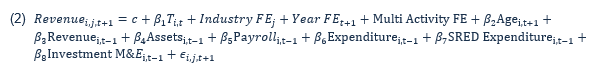
Text version
Revenue of firm i, in industry j, at time t plus 1, is equal to a constant, plus the average treatment effect, beta 1, multiplied by the treatment status of firm i, in industry j, at time t, plus the industry fixed effect, plus the year fixed effect, plus the multi activity flag, plus the beta 2 multiplied by the age of firm i, in industry j, at time t - 1, plus beta 3 multiplied by the revenue age of firm i, in industry j, at time t - 1, plus beta 4 multiplied by assets age of firm i, in industry j, at time t - 1, plus beta five multiplied by payroll age of firm i, in industry j, at time t - 1, plus beta 6 multiplied by expenditures age of firm i, in industry j, at time t - 1, plus beta 7 multiplied by the SRED expenditure age of firm i, in industry j, at time t - 1, plus beta 8 multiplied by the investment in M&E of age of firm i, in industry j, at time t - 1, plus an error term of age of firm i, in industry j, at time t + 1.
As a second example, using assets five-years after the CTA program:
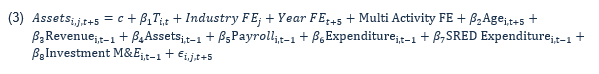
Text version
Assets of firm i, in industry j, at time t plus 5, is equal to a constant, plus the average treatment effect, beta 1, multiplied by the treatment status of firm i, in industry j, at time t, plus the industry fixed effect, plus the year fixed effect, plus the multi activity flag, plus the beta 2 multiplied by the age of firm i, in industry j, at time t - 1, plus beta 3 multiplied by the revenue age of firm i, in industry j, at time t - 1, plus beta 4 multiplied by assets age of firm i, in industry j, at time t - 1, plus beta five multiplied by payroll age of firm i, in industry j, at time t - 1, plus beta 6 multiplied by expenditures age of firm i, in industry j, at time t - 1, plus beta 7 multiplied by the SRED expenditure age of firm i, in industry j, at time t - 1, plus beta 8 multiplied by the investment in M&E of age of firm i, in industry j, at time t - 1, plus an error term of age of firm i, in industry j, at time t + 5.
While the selection of variables to address the selection bias is the most important, decisions also extend to the model type employed in the estimation. As mentioned above, the first model is simply OLS regression. Subsequently, three matching methods, detailed below, are implemented. Considering that all four methods are valid causal techniques conditional on covariates, they are expected to yield similar estimates when the right set of covariates is chosen.
- A) Propensity score matching
Propensity score matching is the most common type of matching.Footnote 12 Footnote 13 It operates as a two-stage estimator. In the first stage, a probit or logistic regression is run to estimate the probability of firms being selected into treatment, generating fitted values known as propensity score. Subsequently, using these propensity scores, each treated observation is paired with a control observation.Footnote 14 In the second stage, a weighted regression is run with the weights corresponding to the matched observations.
Despite being the most popular type of matching, propensity score matching may not be the most appropriate type of matching to alleviate endogeneity concerns. Propensity scores condense all of the information in the covariates into a single dimension—the fitted value. Consequently, it is conceivable that firms could have a similar fitted value, without possessing comparable characteristics. Despite the intention of propensity scores to reduce the imbalance between treated and control groups, in some cases propensity scores instead exacerbate the imbalance. A more thorough examination of the issues of propensity score matching can be found in King & Neilsen.Footnote 15
- B) Inverse-probability weighted matching
Inverse probability weighting is similar to propensity score matching, but it makes “weird” observations more important. Instead of using the propensity score as weights, it uses the treatment status divided by the propensity score as weights.Footnote 16 Footnote 17 The formula for the inverse probability weight (when the outcome is binary) is expressed in equation (3):
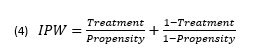
Text version
The inverse probability weight is equal to treatment divided by propensity plus 1 minus treatment divided by 1 minus propensity.
Having the propensity scores in the denominator implies that whenever an observation is treated when the propensity score is low (or is untreated when the propensity score is high), that observation will have a greater weight than observations exhibiting the anticipated behaviour. There is some evidence that inverse probability weighting performs better than propensity score weighting on simulated data.Footnote 18
- C) Robust Mahalanobis matching
In contrast to using a first stage regression and using propensity scores, Mahalanobis matching relies on constructing the Mahalanobis distance between two observations.Footnote 19 Because the distance is derived directly from the covariates themselves, rather than the estimated propensity score, the matched pairs are more likely to exhibit close values on the covariates, facilitating potentially improved comparisons. King and Neilsen (2019) advocate for Mahalanobis matching over propensity score matching based on this argument.
The robust version of Mahalanobis matching is computed not on the covariates directly, but rather on their ranks.Footnote 20 Footnote 21 Given the purpose of the robust Mahalanobis distance is to calculate the distance between variables, it follows that it is commonly used as a method for detecting outliers in statistics.Footnote 22 While most recent literature tends to align with King and Neilsen, there are dissenting viewpoints. For instance, Ripollone et al. (2018), contend that propensity score matching is still a useful estimating technique.Footnote 23
Given the lack of consensus on which matching strategy is preferred, this paper employs all three. However, in alignment with the arguments put forth by King and Neilsen, the robust Mahalanobis method is considered the preferred approach. There are additional matching estimators that are available such as: regression adjustment, augment inverse probability weighting, inverse probability weighting with regression adjustment, among others.Footnote 24 Unfortunately, these techniques were unavailable at the time due to limitations on computational power.
Another decision involves determining the number of observations to match with each observation in the treated group. Common choices include nearest neighbour (1:1 matching); k:1 matching; and full matching (matching with each observation with all observations).Footnote 25 Rosenbaum (2020) contends that due to diminishing returns, there is limited precision gain beyond matching on four control observations.Footnote 26 Consequently, propensity score matching and robust Mahalanobis matching in this study are executed with five observations. The inverse probability weighting method uses all observations.
Additional matching options include optimal matching, greedy matching, and coarsened exact matching. Unfortunately, limitations on computation power prevented full matching, or optimal matching with the robust Mahalanobis method. Thus, the propensity score is optimal matching on five control observations, while the robust Mahalanobis is greedy matching on five control observations.
4. Results from OLS and Matching
The regression results are presented in the appendix in tables 4-9, revealing consistently positive outcomes for firms that participated in the CTA program compared to those that did not. To offer an interpretation of table 4, column 7 (the average treatment effect with robust Mahalanobis matching), the revenue of a firm one-year after the CTA program is 27%Footnote 27 greater than that of comparable firms that did not participate in the program. These comparable firms were selected based on being in the same industry and year, and then further matched for similarity in factors such as operating in multiple industries (or not), similar ages, and comparable values of: revenue, assets, payroll, expenditure, SRED expenditure, and investment in machinery and equipment, in the year prior to the firm entering the CTA. As time progresses, the positive impact persists. Three years after the program, the revenue differential widens to 55%, and after five years, the revenue for firms in the CTA program surpasses that of non-participating firms by 129%.
To quantify the monetary impact of the program on firm revenue, a simple approach involves multiplying the estimate for the average treatment effect on the treated (ATT) by the mean firm size. Utilizing the ATT is more appropriate in this context than the average treatment effect (ATE), as it specifically estimates the program's effectiveness on treated firms. However, it’s important to note that this method only provides a rough estimate. The main caveat which renders this a crude estimate is that it ignores heterogeneous treatment effects based on firm size. The econometric estimates deliver an average treatment effect as a percentage difference, without considering potential changes in the effect as firms vary in size. Moreover, given the significant standard deviation in the average firm size (as indicated in table 1), there exists considerable variability in firm sizes, ranging from much smaller to much larger entities compared to the mean. Despite these considerations, evaluating the ATT estimate from the Mahalanobis matching of 37.7%Footnote 28 at the mean of revenue of $3.5 million, suggests that the average effect of the CTA program is a $1.3 million increase in revenue per firm after one year.
Three overarching trends are discernible across all the results. Firstly, the estimates are almost all positive and statistically significant. Secondly, the coefficients consistently become larger as more time elapses following the completion of the CTA program. This could be interpreted as not only the CTA program having a sustained impact, but also a realization of the program’s benefits over an extended period. Thirdly, the ATT is consistently stronger than the ATE.Footnote 29 A possible interpretation is to imply that the CTA program yields benefits across all firms in the analyzed subset of industries (the ATE), but has a greater benefit to the firms that have the characteristics of a typical firm that has completed the CTA program (the ATT).
It is noteworthy that the coefficients are stable across estimators. In general, all the matching estimators tend to have coefficients that have magnitudes that are relatively close to one-another, irrespective of whether the focus is on estimating the ATE or the ATT. Even the OLS with all controls included yields estimates that align with the matching estimates. This congruence in results is a positive feature. If both OLS (which projects the treatment effect into the span orthogonal to the other regressors) and matching estimators (which compares the treated firm with untreated firms that have similar characteristics) provide causal estimates, conditional on covariates, then they should produce similar results if the appropriate conditioning has been applied.
The results demonstrate the most robust effects for expenditures and SRED expenditures, while indicating comparatively weaker impacts for investment in machinery and equipment. For expenditures and SRED expenditures, positive and statistically significant coefficients persist across various time frames, estimators, and whether estimating the ATE or ATT. Conversely, for investment in machinery and equipment, statistically significant coefficients emerge only 5-years after the completion of the program, with the evidence appearing less robust compared to other variables.
For revenue, assets, and payroll, most coefficients are positive and statistically significant. Notably, the exception for all three variables is observed in the average treatment effect using inverse probability weighted matching. A strict interpretation might suggest weaker evidence of an average treatment effect of the CTA program, though the average treatment effect on the treated remains. Alternatively, a more lenient interpretation posits that, given the other consistently positive and statistically significant coefficients, this is an outlier method which does not align with the overall body of evidence.
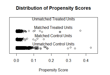
One of the concerns with the propensity score matching arises from the limited participation of firms in the CTA program, leading to a sample imbalance and low fitted propensity scores. Figure 1 presents a jitter plot illustrating the distribution of propensity scores among the treated, control, and unmatched control firms.
Figure 1: Jitter plot of propensity-score distribution for revenue one year after the CTA programFootnote 30
Text version
Figure 1 shows that most matched treated and control units have a low propensity around 0.05. A few units have higher propensities around 0.1, and very few have propensities are higher. For the unmatched control units, most are between 0 and 0.1. A few are higher and between 0. 1 and 0.2 Very few are higher than 0.2, but 3 are about 0.3 and one is above 0.4. There are no unmatched treated units.
A limited number of firms exhibit propensity scores above 0.1, with the majority having scores around 0.05. The concern here lies in the low propensity scores, posing a challenge for propensity score matching. The issue arises because the covariates used for matching may not serve as effective predictors of program entry, given the small size of the program relative to the overall population of firms, rendering it difficult to identify strong predictors. Consequently, matching based on propensity scores presents potential challenges for both propensity score matching and inverse probability weighted matching.
However, these concerns are mitigated by the application of the robust Mahalanobis matching. Since robust Mahalanobis matching relies on the closeness of the variables rather than the propensity score, the issue of low propensity scores is circumvented. Given the similarity of results despite the different matching methods, it appears that in this instance, the low propensity scores did not pose a significant issue.
5. Fixed-effects regression
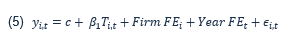
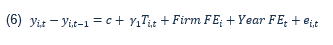
To address lingering endogeneity concerns, supplementary regressions were conducted by introducing firm and year fixed-effects. Until this point in the analysis, all the variation has originated from differences between firms. CTA firms have been compared to non-CTA firms to establish the counterfactual. However, considering the longitudinal nature of the NALMF dataset, an additional source of valuable variation arises from within the same firm, pre- and post-CTA. This approach aids in alleviating concerns of selection bias, as it involves comparing the firms against themselves over time.
The first regression, expressed in equation (5), was on the natural log level of the outcomes of interest, where the CTA variable equals zero prior to the firm entering the CTA, and equals one after completing the program. This regression captures whether firms exhibit higher outcomes post-CTA compared to pre-CTA. The second regression, in equation (6), was performed on the differences in the natural log level, capturing whether the growth in those variables increased post-CTA relative to pre-CTA.
Text version
Equation 5 is the outcome of firm i at time t is equal to a constant plus beta 1 multiplied by the treatment status of firm i at time t, plus the firm i fixed effect, plus the year t fixed effect, plus an error term of firm i at time t.
Text version
Equation 6 is the outcome of firm i at time t minus the outcome of firm i at time t minus one, is equal to a constant plus beta 1 multiplied by the treatment status of firm i at time t, plus the firm i fixed effect, plus the year t fixed effect, plus an error term of firm i at time t.
Given that the variation in the variable of interest arises exclusively from firms that participated in the CTA, the sample is limited to firms that at some point participated in the CTA. The results can be found in table 10.
With the exception of investment in machinery and equipment, the results are unambiguous in terms of level—firms exhibit improved outcomes after the CTA compared to before the program. Post-CTA, firms have higher revenue, assets, payroll, expenditure, and SRED expenditure compared to the pre-CTA period. However, there is some evidence that the growth of these variables tends to decelerate post-CTA compared to pre-CTA.
While it would have significantly bolstered the case for the effectiveness of the CTA program if the results of the second set of fixed-effects regressions were positive, the fact that many of the results are negative and statistically significant is not necessarily a drawback. It is crucial to consider that one of the criteria for qualifying into the CTA is being a fast-growing firm before entering the program. It is reasonable to anticipate that the growth of fast-growing firms may naturally decelerate over time. There are several studies that show as firm size is negatively correlated with firm growth (e.g Hölzl (2009), Levratto et al. (2010)), and other literature that finds that the autocorrelation of firm growth is negative and high growth does not exhibit persistence (Coad et al. 2014). In general, as firms grow and become larger, their growth naturally slows down.
Determining the counterfactual scenario of how fast firms would grow in the absence of the CTA can be approached in two ways. The first involves constructing a structural model of firm growth, a task beyond the scope of this analysis. The second method entails comparing CTA firms with non-CTA firms to discern the differences in outcomes. A viable approach for the second method is to utilize a matching strategy, akin to the methodology employed in the preceding section. In this strategy, one of the matching criteria is the growth of firms pre-CTA, with the outcome being the growth of firms post-CTA. Although attempted, the results yielded a mixed picture, with some indicating positive effects, the majority showing no statistically significant differences from zero, and others displaying negative effects. However, it's important to note that the sample size was insufficient to draw robust conclusions from these findings.
6. Conclusion
This paper has attempted to provide a causal estimate of the CTA program on firms. Prior research, and the growth comparison presented in this paper, establish that CTA-participating firms exhibit superior outcomes compared to their non-CTA counterparts. However, the lingering question has been whether these positive results can be attributed to the CTA program or if the program administrators are adept at selecting inherently successful firms, irrespective of their participation in the CTA program.
Using various matching estimators and matching on industry, year, age, and pre-treatment outcomes to address the selection bias, this analysis concludes that the Canadian Technology Accelerator program has a positive causal effect on firm outcomes. Specifically, the CTA program causes firm revenue to increase by 27% in the year after the CTA, compared to non-CTA participating firms that otherwise have similar characteristics. Similar positive effects are observed for assets, payroll, expenditures, and SRED expenditures. These outcomes are stable across different estimators and strengthen over time after program completion. Using firm fixed-effects to change the variation from inter-firm to intra-firm finds similar positive results of the program. While the analysis reveals a deceleration in growth after the program, this might be attributed to the natural slowdown of fast-growing firms. Estimating the counterfactual of firm growth in the context of the CTA is a potential avenue for future research.
These results validate and strengthen previous conclusions about CTA firms achieving increased revenue, obtaining new capital, and creating employment. While one of the primary goals of the CTA program is to support the international growth of clients, data limitations hindered an exploration of international expansion, leaving it as another potential area for future research. Nevertheless, the positive outcomes attributable to the CTA program, as highlighted here, underscore its effectiveness.
7. Appendix with econometric results
Table 4: Results from regression with Revenue as the dependent variable
| OLS | OLS with controls | IPW ATE | IPW ATT | Propensity Score ATE | Propensity Score ATT | Mahalanobis ATE | Mahalanobis ATT | |
|---|---|---|---|---|---|---|---|---|
| 1-year | 1.62 | 0.42 | 0.11 | 0.28 | 0.19 | 0.33 | 0.24 | 0.32 |
| SE | 0.09 | 0.14 | 0.13 | 0.08 | 0.07 | 0.08 | 0.06 | 0.07 |
| T-stat | 17.6 | 3.01 | 0.85 | 3.63 | 2.71 | 4.23 | 3.75 | 4.74 |
| P-value | 0 | 0 | 0.4 | 0 | 0.007 | 0 | 0 | 0 |
| N | 5,074,838 | 61,225 | 47,601 | 47,601 | ||||
| N-treated | 192 | 192 | 192 | 192 | ||||
| 3-years | 1.98 | 0.62 | 0.2 | 0.43 | 0.42 | 0.55 | 0.44 | 0.48 |
| SE | 0.14 | 0.08 | 0.22 | 0.14 | 0.13 | 0.14 | 0.13 | 0.14 |
| T-stat | 14.15 | 7.52 | 0.93 | 3.19 | 3.36 | 4.09 | 3.41 | 3.44 |
| P-value | 0 | 0 | 0.35 | 0 | 0.001 | 0 | 0.001 | 0.001 |
| N | 3,071,354 | 41,398 | 29,553 | 29,553 | ||||
| N-treated | 118 | 118 | 118 | 118 | ||||
| 5-years | 2.13 | 1.1 | 0.53 | 0.94 | 0.81 | 0.88 | 0.83 | 0.9 |
| SE | 0.24 | 0.15 | 0.32 | 0.2 | 0.17 | 0.15 | 0.18 | 0.15 |
| T-stat | 8.95 | 7.26 | 1.65 | 4.79 | 4.63 | 5.81 | 4.71 | 5.91 |
| P-value | 0 | 0 | 0.1 | 0 | 0 | 0 | 0 | 0 |
| N | 1,590,271 | 23,656 | 15,131 | 15,131 | ||||
| N-treated | 75 | 75 | 75 | 75 |
Notes: The rows “1-year”, “3-years”, and “5-years” contain the coefficients on the variable “CTA Client” 1-year, 3-years, and 5-years, respectively, after the firm has completed the CTA program. The bolded coefficients are significant at the 5% level. The dependent variable is measured in natural log. N is the total sample size for the regression, N-treated is the number of different firms. The reasons for the differences in reporting have to do with Stata vs R-studio.
The control variables, and the variables used in matching, were an industry dummy variable, a year dummy variable, a multi-activity dummy variable, the age of the firm, the natural log of revenue 1-year prior to the CTA, the natural log of assets 1-year prior to the CTA, the natural log of payroll 1-year prior to the CTA, the natural log of expenses 1-year prior to the CTA, the natural log of SRED expenditure 1-year prior to the CTA, and the natural log of investment in machinery and equipment 1-year prior to the CTA.
The first column is an OLS with only the CTA-client variable included, with robust standard errors. The second column is OLS with all of the control variables, with standard errors clustered on industry id. The third column is the average treatment effect from inverse-probability weighted matching. The fourth column is the average treatment effect on the treated from inverse-probability weighted matching. The fifth column is the average treatment effect from propensity-score matching. The sixth column is the average treatment effect on the treated from propensity-score matching. The seventh column is the average treatment effect from Mahalanobis matching. The eighth column is the average treatment effect on the treated from Mahalanobis matching.
The 27% increase in revenue after one-year comes from the coefficient on Mahalanobis ATE, calculated as . Likewise, the 37.7% from the Mahalanobis ATT coefficient is calculated as .
Table 5: Results from regression with Assets as the dependent variable
| OLS | OLS with controls | IPW ATE | IPW ATT | Propensity Score ATE | Propensity Score ATT | Mahalanobis ATE | Mahalanobis ATT | |
|---|---|---|---|---|---|---|---|---|
| 1-year | 1.66 | 0.36 | 0.22 | 0.32 | 0.24 | 0.27 | 0.31 | 0.33 |
| SE | 0.09 | 0.07 | 0.15 | 0.08 | 0.07 | 0.08 | 0.08 | 0.07 |
| T-stat | 17.78 | 5.46 | 1.47 | 3.93 | 3.37 | 3.46 | 4.1 | 4.38 |
| P-value | 0 | 0 | 0.141 | 0 | 0.001 | 0.001 | 0 | 0 |
| N | 5,783,264 | 61,818 | 48,107 | 48,107 | ||||
| N-treated | 193 | 193 | 193 | 193 | ||||
| 3-years | 1.75 | 0.47 | -0.01 | 0.4 | 0.31 | 0.44 | 0.36 | 0.45 |
| SE | 0.14 | 0.11 | 0.26 | 0.13 | 0.14 | 0.13 | 0.12 | 0.12 |
| T-stat | 12.41 | 4.39 | -0.04 | 3.17 | 2.23 | 3.26 | 2.89 | 3.87 |
| P-value | 0 | 0 | 0.969 | 0.002 | 0.025 | 0.001 | 0.004 | 0 |
| N | 3,486,515 | 42,090 | 30,096 | 30,096 | ||||
| N-treated | 118 | 118 | 118 | 118 | ||||
| 5-years | 2.05 | 0.86 | 0.36 | 0.78 | 0.67 | 0.78 | 0.88 | 0.88 |
| SE | 0.21 | 0.2 | 0.29 | 0.21 | 0.2 | 0.18 | 0.2 | 0.19 |
| T-stat | 9.8 | 4.4 | 1.25 | 3.77 | 3.35 | 4.29 | 4.38 | 4.73 |
| P-value | 0 | 0 | 0.211 | 0 | 0.001 | 0 | 0 | 0 |
| N | 1,797,983 | 24,211 | 15,549 | 15,549 | ||||
| N-treated | 75 | 75 | 75 | 75 |
Notes: The rows “1-year”, “3-years”, and “5-years” contain the coefficients on the variable “CTA_Client” 1-year, 3-years, and 5-years, respectively, after the firm has completed the CTA program. The bolded coefficients are significant at the 5% level. The dependent variable is measured in natural log. N is the total sample size for the regression, N-treated is the number of different firms. The reasons for the differences in reporting have to do with Stata vs R-studio.
The control variables, and the variables used in matching, were an industry dummy variable, a year dummy variable, a multi-activity dummy variable, the age of the firm, the natural log of revenue 1-year prior to the CTA, the natural log of assets 1-year prior to the CTA, the natural log of payroll 1-year prior to the CTA, the natural log of expenses 1-year prior to the CTA, the natural log of SRED expenditure 1-year prior to the CTA, and the natural log of investment in machinery and equipment 1-year prior to the CTA.
The first column is an OLS with only the CTA-client variable included, with robust standard errors. The second column is OLS with all of the control variables, with standard errors clustered on industry id. The third column is the average treatment effect from inverse-probability weighted matching. The fourth column is the average treatment effect on the treated from inverse-probability weighted matching. The fifth column is the average treatment effect from propensity-score matching. The sixth column is the average treatment effect on the treated from propensity-score matching. The seventh column is the average treatment effect from Mahalanobis matching. The eighth column is the average treatment effect on the treated from Mahalanobis matching.
Table 6: Results from regressions Payroll with as the dependent variable
| OLS | OLS with controls | IPW ATE | IPW ATT | Propensity Score ATE | Propensity Score ATT | Mahalanobis ATE | Mahalanobis ATT | |
|---|---|---|---|---|---|---|---|---|
| 1-year | 1.93 | 0.35 | -0.02 | 0.27 | 0.16 | 0.25 | 0.21 | 0.31 |
| SE | 0.07 | 0.07 | 0.2 | 0.08 | 0.08 | 0.07 | 0.11 | 0.07 |
| T-stat | 25.71 | 5.26 | -0.11 | 3.43 | 2 | 3.45 | 1.9 | 4.28 |
| P-value | 0 | 0 | 0.916 | 0.001 | 0.046 | 0.001 | 0.057 | 0 |
| N | 2,871,301 | 60,468 | 46,987 | 46,987 | ||||
| N-treated | 195 | 195 | 195 | 195 | ||||
| 3-years | 2.25 | 0.61 | 0.26 | 0.52 | 0.39 | 0.5 | 0.55 | 0.62 |
| SE | 0.10 | 0.09 | 0.21 | 0.1 | 0.07 | 0.07 | 0.07 | 0.08 |
| T-stat | 21.96 | 6.84 | 1.22 | 5.34 | 5.31 | 6.93 | 7.63 | 8 |
| P-value | 0 | 0 | 0.223 | 0 | 0 | 0 | 0 | 0 |
| N | 1,761,819 | 39,929 | 28,334 | 28,334 | ||||
| N-treated | 113 | 113 | 113 | 113 | ||||
| 5-years | 2.45 | 0.65 | 0.48 | 0.51 | 0.23 | 0.39 | 0.52 | 0.55 |
| SE | 0.15 | 0.19 | 0.25 | 0.18 | 0.15 | 0.15 | 0.14 | 0.13 |
| T-stat | 16.6 | 3.39 | 1.89 | 2.87 | 1.48 | 2.66 | 3.7 | 4.13 |
| P-value | 0 | 0.001 | 0.059 | 0.004 | 0.138 | 0.008 | 0 | 0 |
| N | 925,934 | 22,517 | 14,232 | 14,232 | ||||
| N-treated | 70 | 70 | 70 | 70 |
Notes: The rows “1-year”, “3-years”, and “5-years” contain the coefficients on the variable “CTA_Client” 1-year, 3-years, and 5-years, respectively, after the firm has completed the CTA program. The bolded coefficients are significant at the 5% level. The dependent variable is measured in natural log. N is the total sample size for the regression, N-treated is the number of different firms. The reasons for the differences in reporting have to do with Stata vs R-studio.
The control variables, and the variables used in matching, were an industry dummy variable, a year dummy variable, a multi-activity dummy variable, the age of the firm, the natural log of revenue 1-year prior to the CTA, the natural log of assets 1-year prior to the CTA, the natural log of payroll 1-year prior to the CTA, the natural log of expenses 1-year prior to the CTA, the natural log of SRED expenditure 1-year prior to the CTA, and the natural log of investment in machinery and equipment 1-year prior to the CTA.
The first column is an OLS with only the CTA-client variable included, with robust standard errors. The second column is OLS with all of the control variables, with standard errors clustered on industry id. The third column is the average treatment effect from inverse-probability weighted matching. The fourth column is the average treatment effect on the treated from inverse-probability weighted matching. The fifth column is the average treatment effect from propensity-score matching. The sixth column is the average treatment effect on the treated from propensity-score matching. The seventh column is the average treatment effect from Mahalanobis matching. The eighth column is the average treatment effect on the treated from Mahalanobis matching.
Table 7: Results from regressions with Expenditures as the dependent variable
| OLS | OLS with controls | IPW ATE | IPW ATT | Propensity Score ATE | Propensity Score ATT | Mahalanobis ATE | Mahalanobis ATT | |
|---|---|---|---|---|---|---|---|---|
| 1-year | 3.22 | 0.51 | 0.3 | 0.46 | 0.4 | 0.46 | 0.39 | 0.43 |
| SE | 0.08 | 0.06 | 0.1 | 0.05 | 0.05 | 0.05 | 0.06 | 0.05 |
| T-stat | 42.75 | 8.83 | 2.93 | 8.66 | 7.68 | 8.86 | 6.93 | 8.8 |
| P-value | 0 | 0 | 0.003 | 0 | 0 | 0 | 0 | 0 |
| N | 5,468,004 | 61,712 | 48,022 | 48,022 | ||||
| N-treated | 194 | 194 | 194 | 194 | ||||
| 3-years | 3.4 | 0.67 | 0.41 | 0.64 | 0.61 | 0.71 | 0.6 | 0.63 |
| SE | 0.11 | 0.07 | 0.18 | 0.11 | 0.1 | 0.1 | 0.1 | 0.1 |
| T-stat | 29.8 | 9.96 | 2.33 | 5.77 | 5.82 | 7.35 | 5.84 | 6.33 |
| P-value | 0 | 0 | 0.02 | 0 | 0 | 0 | 0 | 0 |
| N | 3,312,695 | 41,950 | 29,989 | 29,989 | ||||
| N-treated | 118 | 118 | 118 | 118 | ||||
| 5-years | 3.49 | 0.98 | 0.57 | 0.96 | 0.84 | 0.86 | 1.03 | 1.04 |
| SE | 0.18 | 0.14 | 0.23 | 0.17 | 0.15 | 0.14 | 0.16 | 0.15 |
| T-stat | 19.09 | 7.04 | 2.45 | 5.55 | 5.65 | 6.01 | 6.34 | 7.07 |
| P-value | 0 | 0 | 0.014 | 0 | 0 | 0 | 0 | 0 |
| N | 1,712,438 | 24,095 | 15,460 | 15,460 | ||||
| N-treated | 75 | 75 | 75 | 75 |
Notes: The rows “1-year”, “3-years”, and “5-years” contain the coefficients on the variable “CTA_Client” 1-year, 3-years, and 5-years, respectively, after the firm has completed the CTA program. The bolded coefficients are significant at the 5% level. The dependent variable is measured in natural log. N is the total sample size for the regression, N-treated is the number of different firms. The reasons for the differences in reporting have to do with Stata vs R-studio.
The control variables, and the variables used in matching, were an industry dummy variable, a year dummy variable, a multi-activity dummy variable, the age of the firm, the natural log of revenue 1-year prior to the CTA, the natural log of assets 1-year prior to the CTA, the natural log of payroll 1-year prior to the CTA, the natural log of expenses 1-year prior to the CTA, the natural log of SRED expenditure 1-year prior to the CTA, and the natural log of investment in machinery and equipment 1-year prior to the CTA.
The first column is an OLS with only the CTA-client variable included, with robust standard errors. The second column is OLS with all of the control variables, with standard errors clustered on industry id. The third column is the average treatment effect from inverse-probability weighted matching. The fourth column is the average treatment effect on the treated from inverse-probability weighted matching. The fifth column is the average treatment effect from propensity-score matching. The sixth column is the average treatment effect on the treated from propensity-score matching. The seventh column is the average treatment effect from Mahalanobis matching. The eighth column is the average treatment effect on the treated from Mahalanobis matching.
Table 8: Results from regressions with SRED Expenditures as the dependent variable
| OLS | OLS with controls | IPW ATE | IPW ATT | Propensity Score ATE | Propensity Score ATT | Mahalanobis ATE | Mahalanobis ATT | |
|---|---|---|---|---|---|---|---|---|
| 1-year | 1.58 | 0.33 | 0.41 | 0.31 | 0.2 | 0.25 | 0.25 | 0.3 |
| SE | 0.07 | 0.84 | 0.15 | 0.07 | 0.06 | 0.06 | 0.08 | 0.07 |
| T-stat | 21.19 | 3.94 | 2.74 | 4.5 | 3.23 | 3.86 | 3.21 | 4.59 |
| P-value | 0 | 0 | 0.006 | 0 | 0.001 | 0 | 0.001 | 0 |
| N | 93,771 | 47,814 | 37,750 | 37,750 | ||||
| N-treated | 177 | 177 | 177 | 177 | ||||
| 3-years | 2.13 | 0.46 | 0.77 | 0.43 | 0.36 | 0.43 | 0.46 | 0.48 |
| SE | 0.10 | 0.09 | 0.32 | 0.1 | 0.08 | 0.08 | 0.09 | 0.09 |
| T-stat | 21.61 | 5.18 | 2.43 | 4.42 | 4.49 | 5.4 | 5.32 | 5.29 |
| P-value | 0 | 0 | 0.015 | 0 | 0 | 0 | 0 | 0 |
| N | 59,441 | 27,557 | 19,725 | 19,725 | ||||
| N-treated | 97 | 97 | 97 | 97 | ||||
| 5-years | 2.57 | 0.59 | 0.62 | 0.56 | 0.48 | 0.5 | 0.6 | 0.56 |
| SE | 0.13 | 0.11 | 0.21 | 0.15 | 0.09 | 0.08 | 0.13 | 0.13 |
| T-stat | 20.63 | 5.3 | 3.03 | 3.87 | 5.24 | 6.23 | 4.72 | 4.37 |
| P-value | 0 | 0 | 0.002 | 0 | 0 | 0 | 0 | 0 |
| N | 31,621 | 13,860 | 8,887 | 8,887 | ||||
| N-treated | 58 | 58 | 58 | 58 |
Notes: The rows “1-year”, “3-years”, and “5-years” contain the coefficients on the variable “CTA_Client” 1-year, 3-years, and 5-years, respectively, after the firm has completed the CTA program. The bolded coefficients are significant at the 5% level. The dependent variable is measured in natural log. N is the total sample size for the regression, N-treated is the number of different firms. The reasons for the differences in reporting have to do with Stata vs R-studio.
The control variables, and the variables used in matching, were an industry dummy variable, a year dummy variable, a multi-activity dummy variable, the age of the firm, the natural log of revenue 1-year prior to the CTA, the natural log of assets 1-year prior to the CTA, the natural log of payroll 1-year prior to the CTA, the natural log of expenses 1-year prior to the CTA, the natural log of SRED expenditure 1-year prior to the CTA, and the natural log of investment in machinery and equipment 1-year prior to the CTA.
The first column is an OLS with only the CTA-client variable included, with robust standard errors. The second column is OLS with all of the control variables, with standard errors clustered on industry id. The third column is the average treatment effect from inverse-probability weighted matching. The fourth column is the average treatment effect on the treated from inverse-probability weighted matching. The fifth column is the average treatment effect from propensity-score matching. The sixth column is the average treatment effect on the treated from propensity-score matching. The seventh column is the average treatment effect from Mahalanobis matching. The eighth column is the average treatment effect on the treated from Mahalanobis matching.
Table 9: Results from regressions with Investment in M&E as the dependent variable
| OLS | OLS with controls | IPW ATE | IPW ATT | Propensity Score ATE | Propensity Score ATT | Mahalanobis ATE | Mahalanobis ATT | |
|---|---|---|---|---|---|---|---|---|
| 1-year | 1.05 | 0.22 | 0.09 | 0.15 | 0.11 | 0.21 | 0.21 | 0.24 |
| SE | 0.12 | 0.11 | 0.18 | 0.13 | 0.14 | 0.13 | 0.14 | 0.12 |
| T-stat | 8.85 | 2.06 | 0.5 | 1.14 | 0.74 | 1.63 | 1.47 | 1.97 |
| P-value | 0 | 0.043 | 0.617 | 0.255 | 0.462 | 0.103 | 0.141 | 0.049 |
| N | 1,681,160 | 51,910 | 38,714 | 38,714 | ||||
| N-treated | 163 | 163 | 163 | 163 | ||||
| 3-years | 1.38 | 0.24 | -0.17 | 0.15 | 0.08 | 0.17 | 0.11 | 0.16 |
| SE | 0.15 | 0.12 | 0.28 | 0.16 | 0.15 | 0.15 | 0.15 | 0.14 |
| T-stat | 8.93 | 1.97 | -0.61 | 0.94 | 0.55 | 1.16 | 0.71 | 1.19 |
| P-value | 0 | 0.052 | 0.541 | 0.346 | 0.583 | 0.244 | 0.478 | 0.235 |
| N | 1,011,128 | 33,639 | 22,827 | 22,827 | ||||
| N-treated | 98 | 98 | 98 | 98 | ||||
| 5-years | 1.58 | 0.65 | 0.66 | 0.49 | 0.48 | 0.45 | 0.59 | 0.47 |
| SE | 0.25 | 0.25 | 0.26 | 0.27 | 0.22 | 0.22 | 0.27 | 0.22 |
| T-stat | 6.42 | 2.63 | 2.51 | 1.86 | 2.18 | 2.06 | 2.18 | 2.15 |
| P-value | 0 | 0.01 | 0.012 | 0.063 | 0.029 | 0.039 | 0.03 | 0.031 |
| N | 525,177 | 18,756 | 10,786 | 10,786 | ||||
| N-treated | 59 | 59 | 59 | 59 |
Notes: The rows “1-year”, “3-years”, and “5-years” contain the coefficients on the variable “CTA_Client” 1-year, 3-years, and 5-years, respectively, after the firm has completed the CTA program. The bolded coefficients are significant at the 5% level. The dependent variable is measured in natural log. N is the total sample size for the regression, N-treated is the number of different firms. The reasons for the differences in reporting have to do with Stata vs R-studio.
The control variables, and the variables used in matching, were an industry dummy variable, a year dummy variable, a multi-activity dummy variable, the age of the firm, the natural log of revenue 1-year prior to the CTA, the natural log of assets 1-year prior to the CTA, the natural log of payroll 1-year prior to the CTA, the natural log of expenses 1-year prior to the CTA, the natural log of SRED expenditure 1-year prior to the CTA, and the natural log of investment in machinery and equipment 1-year prior to the CTA.
The first column is an OLS with only the CTA-client variable included, with robust standard errors. The second column is OLS with all of the control variables, with standard errors clustered on industry id. The third column is the average treatment effect from inverse-probability weighted matching. The fourth column is the average treatment effect on the treated from inverse-probability weighted matching. The fifth column is the average treatment effect from propensity-score matching. The sixth column is the average treatment effect on the treated from propensity-score matching. The seventh column is the average treatment effect from Mahalanobis matching. The eighth column is the average treatment effect on the treated from Mahalanobis matching.
Table 10: Results from the fixed-effects regressions
| In log levels | Difference in log levels | |
|---|---|---|
| Revenue | 0.164 | -0.1051 |
| SE | 0.073 | 0.063 |
| T-stat | 2.25 | -1.66 |
| P-value | 0.025 | 0.099 |
| N | 2972 | 2472 |
| Assets | 0.186 | -0.0585 |
| SE | 0.0813 | 0.0681 |
| T-stat | 2.29 | -0.86 |
| P-value | 0.022 | 0.391 |
| N | 3069 | 2580 |
| Payroll | 0.185 | -0.185 |
| SE | 0.057 | 0.051 |
| T-stat | 3.25 | -3.63 |
| P-value | 0.001 | 0 |
| N | 2796 | 2311 |
| Expenses | 0.171 | -0.16 |
| SE | 0.073 | 0.0467 |
| T-stat | 2.35 | -3.43 |
| P-value | 0.019 | 0.001 |
| N | 3066 | 2576 |
| SRED Exp | 0.126 | -0.176 |
| SE | 0.0585 | 0.063 |
| T-stat | 2.15 | -2.81 |
| P-value | 0.032 | 0.005 |
| N | 2106 | 1657 |
| Investment ME | -0.0386 | -0.313 |
| SE | 0.12 | 0.153 |
| T-stat | -0.32 | -2.05 |
| P-value | 0.748 | 0.041 |
| N | 2105 | 1560 |
Notes: The variable in the left column is the dependent variable for each regression. The displayed coefficients are on the variable post-CTA which equals 1 after the firm has gone through the CTA program, and 0 prior to the CTA program. The standard errors are clustered by firm. The bolded coefficients are significant at the 5% level.
8. References
Angrist, J. D., & Pischke, J. S. (2009). Mostly harmless econometrics: An empiricist's companion. Princeton university press.
Brookhart, M. A., Schneeweiss, S., Rothman, K. J., Glynn, R. J., Avorn, J., & Stürmer, T. (2006). Variable selection for propensity score models. American journal of epidemiology, 163(12), 1149-1156.
Cabana, E., Lillo, R. E., & Laniado, H. (2021). Multivariate outlier detection based on a robust Mahalanobis distance with shrinkage estimators. Statistical papers, 62, 1583-1609.
Cerulli, G. 2014. treatrew: A user-written command for estimating average treatment effects by reweighting on the propensity score. Stata Journal 14: 541–561.
Chesnaye, Nicholas C., Vianda S. Stel, Giovanni Tripepi, Friedo W. Dekker, Edouard L. Fu, Carmine Zoccali, and Kitty J. Jager. "An introduction to inverse probability of treatment weighting in observational research." Clinical Kidney Journal 15, no. 1 (2022): 14-20.
Coad, A., Daunfeldt, S.-O., Hölzl, W., Johansson, D., and Nightingale, P. (2014). Highgrowth firms: Introduction to the special section. Industrial and Corporate Change, 23(1), 91–112.
Greifer, N. (2023). Matching Methods. MatchIt: Nonparametric Preprocessing for Parametric Causal Inference. Available online: https://cran. r-project. org/web/packages/MatchIt/vignettes/estimating-effects. html (accessed on 30 November 2023).
Heckman, J. J., Ichimura, H., & Todd, P. E. (1997). Matching as an econometric evaluation estimator: Evidence from evaluating a job training programme. The review of economic studies, 64(4), 605-654.
Heckman, J. J., Ichimura, H., & Todd, P. (1998). Matching as an econometric evaluation estimator. The review of economic studies, 65(2), 261-294.
Heiss, Andrew. 2020. “Generating Inverse Probability Weights for Both Binary and Continuous Treatments.” December 1, 2020. https://doi.org/10.59350/1svkc-rkv91.
Hölzl, W. (2009). Is the R&D behaviour of fast-growing SMEs different? Evidence from CIS III data for 16 countries. Small Business Economics, 33(1), 59–75.
King, G., & Nielsen, R. (2019). Why propensity scores should not be used for matching. Political analysis, 27(4), 435-454.
Levratto, N., Tessier, L., and Zouikri, M. (2010). The Determinants of Growth for SMEs — A Longitudinal Study from French Manufacturing Firms. SSRN Electronic Journal, 1780466.
Pearl, J. (2009). Causal inference in statistics: An overview.
Ripollone, John E., Krista F. Huybrechts, Kenneth J. Rothman, Ryan E. Ferguson, and Jessica M. Franklin. 2018. “Implications of the Propensity Score Matching Paradox in Pharmacoepidemiology.” American Journal of Epidemiology 187 (9): 1951-61. https://doi.org/10.1093/aje/kwy078.
Rivard, P. (2020) High-Growth Firm Characteristics In Canada. Ottawa: Innovation, Science and Economic Development Canada.
Rosenbaum, P. R., & Rubin, D. B. (1983). The central role of the propensity score in observational studies for causal effects. Biometrika, 70(1), 41-55.
Rosenbaum, Paul R. 2010. Design of Observational Studies. Springer Series in Statistics. New York: Springer.
Rosenbaum, P. R. (2020). Modern algorithms for matching in observational studies. Annual Review of Statistics and Its Application, 7, 143-176.
Rubin, Donald B. 1980. “Bias Reduction Using Mahalanobis-Metric Matching.” Biometrics 36 (2): 293–98. https://doi.org/10.2307/2529981.
Rubin DB, Thomas N. Matching using estimated propensity scores, relating theory to practice. Biometrics. 1996; 52:249–264.
StataCorp. 2023. Stata 18 Causal Inference and Treatment-Effects Estimation Reference Manual. College Station, TX: Stata Press.
Statistics Canada, National Accounts Longitudinal Microdata File, January 2024. Reproduced and distributed on an "as is" basis with the permission of Statistics Canada.
Statistics Canada, Trade by Exporter Characteristics, January 2024. Reproduced and distributed on an "as is" basis with the permission of Statistics Canada.
Stuart, E. A. (2010). Matching methods for causal inference: A review and a look forward. Statistical science: a review journal of the Institute of Mathematical Statistics, 25(1), 1.
Van Biesebroeck, J., Yu, E., & Chen, S. (2015). The impact of trade promotion services on Canadian exporter performance. Canadian Journal of Economics/Revue canadienne d'économique, 48(4), 1481-1512.
- Date modified: