
Geographic Export Diversity
Colin Scarffe
2019-19-02
Table of Contents
1. Summary
- Canadian merchandise exports are the fourth most concentrated when compared to other countries, but are comparatively less concentrated when destination countries are grouped as regions.
- If the United States is excluded, Canada’s merchandise exports are diversified by country. Canada’s merchandise exports are also diversified by U.S. state.
- Canadian commercial services exports (excluding travel, transportation, and government services) are only moderately less concentrated than Canada’s merchandise exports.
2. Non-technical summary
This study focuses on the diversity of merchandise and commercial services exports by destination. Export diversity is important to hedge against the risk of an economic downturn in partner economies, but it also helps to protect against the threat of trade protectionism. Protectionism is materializing across the world, not only through the United States imposing tariffs on imports of Canadian metal, but also in other events such as Brexit.
Perhaps unsurprisingly, Canadian exports are concentrated because of the high share of its exports that are destined for the United States (U.S.). Out of 113 countries for which merchandise export data for 2017 are available, Canada was the fourth most concentrated behind Kuwait, Bermuda, and Mexico. Canada’s export dependence on the United States is much greater than in economies that have conceivably similar dependence issues, such as Hong Kong with its reliance on China, or New Zealand which depends on Australia.
However, when countries are grouped into regions, both Canada and Mexico are no longer among the most concentrated merchandise exporters. The Scandinavian countries—which have many characteristics similar to the Canadian economy—have a dependency on the European Union (EU) comparable to that of Canada with the United States. Furthermore, when examining individual U.S. states, Canadian exports are no longer concentrated. These two facts suggests that Canada’s trade patterns are actually somewhat normal. The size of the U.S. economy combined with a close proximity, a land border, and the relative costs of exporting elsewhere, mean that Canadian and Mexican exports follow the path of least resistance and are not behaving unnaturally.
Canada’s service exports are also concentrated in the United States. In fact, Canada’s service exports are actually more concentrated than they appear. 55% of Canada’s service exports go to the United States compared to 76% of merchandise exports. This is usually the prime evidence presented when arguing that service exports are more diverse. However, if service exports that are extraneous to trade policy are excluded—travel, transportation, and government services—then 65% of Canada’s (commercial) services exports are destined for the United States. While services exports are still somewhat more diverse than merchandise exports, the gap is smaller than the headline numbers suggest.
3. Introduction
Export diversity can be assessed along multiple dimensions. There is the diversity of what is being exported, the diversity among who is exporting, the diversity of where production takes place, and the diversity of where exports are destined. This study will focus on Canada’s geographic export diversity. The geographic concentration of exports can be problematic because, analogous to a financial portfolio, it is risky to have a single element make up a large share of exports. If a country’s exports are concentrated in a single destination, a recession in that economy, or a bilateral exchange rate shock, would reduce aggregate demand and curtail exports to that country. Exporting to several destinations mitigates the effect of country-specific shocks. A decrease in demand for exports from a country has much different economic implications if that country is the destination of 1% or 50% of exports. It is impossible to diversify away systematic risk—a world recession—but export diversification can temper the effects of country-specific shocks.
In addition to the risks identified above, geographic concentration can expose a country’s exports to the risk of trade protectionism. Protectionism can take the form of tariffs, quotas, non-tariff barriers, dissolution of trade agreements, and other purposely-created hindrances to cross-border commerce and investment. This risk became a reality for Canada when the United States imposed tariffs on Canadian steel and aluminum exports, which came into effect on June 1st, 2018. However, the United States is not the only trade partner of Canada turning towards trade protectionist measures. Another example is the Brexit in the United Kingdom which could eliminate almost half of the EU market for Canadian exports—a market to which Canada was only recently given preferential access under the Canada-European Union Comprehensive Economic and Trade Agreement (CETA).Footnote 1
Diversification of Canadian exports, not only away from the United States, but also across non-U.S. trade partners and the variety of exported products will help shield Canada against the recent trend towards trade protectionism. Not only will it lower the impact of shocks from protectionist measures, but it will also reduce the threat of such measures and give Canada a better bargaining position in trade disputes and negotiations. For instance, if a product-country combination represents an overly large share of exports (for example, Canadian automotive exports to the United States), it gives significantly more clout to the threat of a protectionist measure from the importing country. Thus, greater trade diversification is Canada’s best hedge against both economic shocks and trade protectionism.
The following analysis gives an overview of Canada’s current state of trade diversification by geographic areas and looks at past trends and comparisons with other exporting countries. While the analysis shows that Canada is more diverse than expected, with 76% of exports going to the United States in 2017, there is room for Canada to improve the diversity of its exports across destinations.
4. Merchandise exports by country
By country, Canada’s merchandise exports are not diverse because of the high level of exports destined for the United States.Footnote 2 In 2017, the Herfindahl-Hirschman Index (hereafter HHI) including the United States was 0.58 (concentrated), while the HHI excluding the United States was 0.07 (diverse).Footnote 3 Although the concentration level in 2017 was similar to the level observed in 1990, it has not been stationary. Given the importance of the United States in Canada’s exports, the HHI tracks the U.S. share of Canada’s exports extremely closely—with a correlation of 0.9997. The share of exports destined for the United States increased from 75% in 1990 to just over 87% in 2002. The increasing share of Canada’s exports destined for the United States can be explained, in part, by the strong U.S. economy, the high-tech and auto sector booms, the currency depreciation vis-à-vis the U.S. dollar, and decreased trade barriers from CUSFTA (1987) and NAFTA (1994). After 2002, the concentration and share of exports destined for the United States decreased, reaching a low of 74% in 2011. Reasons for the declining share include faster growing emerging markets, the erosion of Canada-U.S. trade preferences as other free-trade agreements were signed, a currency appreciation against the U.S. dollar, the high-tech bust, a weakening auto sector, a sharp decline in natural gas prices, and the thickening of borders following September 11th. (Brown 2015) Since then, the share of exports destined for the United States has remained relatively steady; in 2017, Canada sent just under 76% of its exports to the United States.
Figure 1: Canada's Merchandise HHI
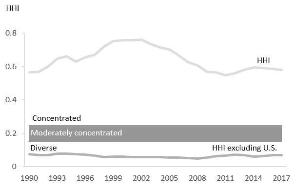
Text version
| Year | HHI | HHI less U.S. | Moderately concentrated | Diverse |
|---|---|---|---|---|
| 1990 | 0.565467 | 0.075395 | 0.25 | 0.15 |
| 1991 | 0.568624 | 0.067623 | 0.25 | 0.15 |
| 1992 | 0.599224 | 0.068165 | 0.25 | 0.15 |
| 1993 | 0.648528 | 0.078085 | 0.25 | 0.15 |
| 1994 | 0.662447 | 0.077605 | 0.25 | 0.15 |
| 1995 | 0.630704 | 0.074433 | 0.25 | 0.15 |
| 1996 | 0.657282 | 0.07051 | 0.25 | 0.15 |
| 1997 | 0.671646 | 0.065121 | 0.25 | 0.15 |
| 1998 | 0.719859 | 0.05795 | 0.25 | 0.15 |
| 1999 | 0.752418 | 0.061297 | 0.25 | 0.15 |
| 2000 | 0.757064 | 0.0612 | 0.25 | 0.15 |
| 2001 | 0.758716 | 0.057703 | 0.25 | 0.15 |
| 2002 | 0.760108 | 0.057268 | 0.25 | 0.15 |
| 2003 | 0.736231 | 0.057656 | 0.25 | 0.15 |
| 2004 | 0.714423 | 0.057226 | 0.25 | 0.15 |
| 2005 | 0.703988 | 0.05501 | 0.25 | 0.15 |
| 2006 | 0.666918 | 0.053356 | 0.25 | 0.15 |
| 2007 | 0.625925 | 0.052651 | 0.25 | 0.15 |
| 2008 | 0.60554 | 0.048561 | 0.25 | 0.15 |
| 2009 | 0.567071 | 0.055089 | 0.25 | 0.15 |
| 2010 | 0.564718 | 0.064525 | 0.25 | 0.15 |
| 2011 | 0.546975 | 0.066541 | 0.25 | 0.15 |
| 2012 | 0.560025 | 0.072923 | 0.25 | 0.15 |
| 2013 | 0.57911 | 0.067997 | 0.25 | 0.15 |
| 2014 | 0.593531 | 0.06095 | 0.25 | 0.15 |
| 2015 | 0.592346 | 0.063505 | 0.25 | 0.15 |
| 2016 | 0.585725 | 0.068878 | 0.25 | 0.15 |
| 2017 | 0.579499 | 0.070272 | 0.25 | 0.15 |
It is useful to compare the level of concentration of Canadian exports with that of other economies. Canadian exports are among the most concentrated of any economy. Canada is 4th on the list behind Kuwait, Bermuda, and Mexico. Footnote 4 Moreover, compared to other economies that are thought to be similar to Canada, such as Hong Kong with its dependence on China or New Zealand with its reliance on Autralia, Canadian exports are much more concentrated.
Figure 2: HHI International Comparisons
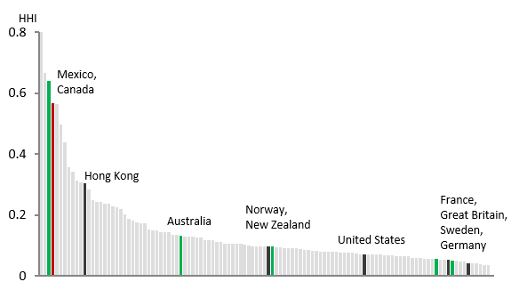
Text version
| Rank | HHI | ISO-3 code | Country |
|---|---|---|---|
| 1 | 0.819362 | KWT | Kuwait |
| 2 | 0.665466 | BMU | Bermuda |
| 3 | 0.641263 | MEX | Mexico |
| 4 | 0.568236 | CAN | Canada |
| 5 | 0.562964 | CPV | Cape Verde |
| 6 | 0.497369 | OMN | Oman |
| 7 | 0.437658 | SLB | Solomon Islands |
| 8 | 0.35643 | NIC | Nicaragua |
| 9 | 0.343298 | NPL | Nepal |
| 10 | 0.312943 | ALB | Albania |
| 11 | 0.307174 | DOM | Dominican Republic |
| 12 | 0.305763 | HKG | Hong Kong, China |
| 13 | 0.284369 | ABW | Aruba |
| 14 | 0.249177 | SLV | El Salvador |
| 15 | 0.244126 | ZMB | Zambia |
| 16 | 0.24215 | PLW | Palau |
| 17 | 0.238425 | MKD | Macedonia, FYR |
| 18 | 0.237265 | JAM | Jamaica |
| 19 | 0.227519 | MLI | Mali |
| 20 | 0.224437 | SUD | Sudan |
| 21 | 0.219535 | BLR | Belarus |
| 22 | 0.203019 | MMR | Myanmar |
| 23 | 0.186508 | HND | Honduras |
| 24 | 0.181792 | BLZ | Belize |
| 25 | 0.175254 | MRT | Mauritania |
| 26 | 0.173925 | MOZ | Mozambique |
| 27 | 0.171538 | WSM | Samoa |
| 28 | 0.151476 | KGZ | Kyrgyz Republic |
| 29 | 0.150932 | BRN | Brunei |
| 30 | 0.149119 | COG | Congo, Rep. |
| 31 | 0.144144 | FJI | Fiji |
| 32 | 0.143121 | BWA | Botswana |
| 33 | 0.142678 | TUN | Tunisia |
| 34 | 0.136006 | PRY | Paraguay |
| 35 | 0.135383 | NAM | Namibia |
| 36 | 0.133191 | AUS | Australia |
| 37 | 0.130036 | CZE | Czech Republic |
| 38 | 0.128305 | AZE | Azerbaijan |
| 39 | 0.12802 | BDI | Burundi |
| 40 | 0.12708 | ARM | Armenia |
| 41 | 0.127079 | ECU | Ecuador |
| 42 | 0.11825 | LUX | Luxembourg |
| 43 | 0.117593 | CHL | Chile |
| 44 | 0.116905 | IRL | Ireland |
| 45 | 0.111319 | ISL | Iceland |
| 46 | 0.110357 | PER | Peru |
| 47 | 0.107024 | MDG | Madagascar |
| 48 | 0.106235 | ISR | Israel |
| 49 | 0.105649 | TZA | Tanzania |
| 50 | 0.105476 | PRT | Portugal |
| 51 | 0.105414 | COL | Colombia |
| 52 | 0.103236 | JOR | Jordan |
| 53 | 0.101116 | URY | Uruguay |
| 54 | 0.097335 | UGA | Uganda |
| 55 | 0.097326 | HUN | Hungary |
| 56 | 0.097197 | POL | Poland |
| 57 | 0.096693 | NZL | New Zealand |
| 58 | 0.096522 | NOR | Norway |
| 59 | 0.095503 | KOR | Korea, Rep. |
| 60 | 0.093002 | GHA | Ghana |
| 61 | 0.092953 | JPN | Japan |
| 62 | 0.092477 | TGO | Togo |
| 63 | 0.091673 | BOL | Bolivia |
| 64 | 0.090694 | MDA | Moldova |
| 65 | 0.090388 | PHL | Philippines |
| 66 | 0.088712 | LKA | Sri Lanka |
| 67 | 0.084385 | SVK | Slovak Republic |
| 68 | 0.084285 | MNT | Montenegro |
| 69 | 0.082798 | ROM | Romania |
| 70 | 0.080976 | DZA | Algeria |
| 71 | 0.080793 | NLD | Netherlands |
| 72 | 0.080367 | BEL | Belgium |
| 73 | 0.079576 | NGA | Nigeria |
| 74 | 0.078694 | KAZ | Kazakhstan |
| 75 | 0.078059 | BIH | Bosnia and Herzegovina |
| 76 | 0.077912 | BRA | Brazil |
| 77 | 0.077904 | SVN | Slovenia |
| 78 | 0.076809 | MUS | Mauritius |
| 79 | 0.07581 | CMR | Cameroon |
| 80 | 0.072291 | EST | Estonia |
| 81 | 0.072054 | USA | United States |
| 82 | 0.072046 | DNK | Denmark |
| 83 | 0.071697 | GEO | Georgia |
| 84 | 0.070522 | SEN | Senegal |
| 85 | 0.069734 | LVA | Latvia |
| 86 | 0.069692 | SGP | Singapore |
| 87 | 0.068889 | MYS | Malaysia |
| 88 | 0.06856 | CYP | Cyprus |
| 89 | 0.067756 | HRV | Croatia |
| 90 | 0.066031 | CHN | China |
| 91 | 0.066011 | CHE | Switzerland |
| 92 | 0.065313 | EUN | European Union |
| 93 | 0.065075 | IDN | Indonesia |
| 94 | 0.060387 | LTU | Lithuania |
| 95 | 0.059418 | SER | Serbia, FR(Serbia/Montenegro) |
| 96 | 0.057755 | ESP | Spain |
| 97 | 0.05622 | RUS | Russian Federation |
| 98 | 0.055746 | PAK | Pakistan |
| 99 | 0.055666 | FRA | France |
| 100 | 0.054609 | FIN | Finland |
| 101 | 0.053713 | BGR | Bulgaria |
| 102 | 0.053383 | KEN | Kenya |
| 103 | 0.053028 | GBR | United Kingdom |
| 104 | 0.051466 | SWE | Sweden |
| 105 | 0.049637 | ARG | Argentina |
| 106 | 0.048468 | IND | India |
| 107 | 0.048467 | ITA | Italy |
| 108 | 0.042784 | DEU | Germany |
| 109 | 0.040399 | EGY | Egypt, Arab Rep. |
| 110 | 0.040215 | ZAF | South Africa |
| 111 | 0.039583 | GRC | Greece |
| 112 | 0.035196 | UKR | Ukraine |
| 113 | 0.035072 | TUR | Turkey |
To some extent, the concentration of Canada’s exports on the United States is predicted by economic theory. The gravity model of trade tells us that economic size and geographic proximity are the most important detminants of bilateral trade patterns. Having a similar culture (language), a land border, and a free-trade agreement further attract Canadian exports to the United States. Also important, there are not many alternatives for Canada’s exports nearby. The country which is closest to Canada in terms of gravity model determinants is Mexico—one of the few countries whose exports are more concentrated than Canada’s. The size of the U.S. economy simply dwarfs all others, and it is thus futile to attempt to make comparisons with other countries’ bilateral relationships.
The reason geographic proximity is included in the gravity model is that the marginal costs of exporting increase the further two countries are separated—consequently, trade is often regional in nature. Furthermore, global value chains are often set up regionally, increasing intra-industry trade within regions.Footnote 5 Thus, simply having more countries in a geographic region may increase trade diversity.
Taking into account the regional dimension, it is also possible to measure trade diversification within geographic regions rather than by country.Footnote 6 By this measure, Canada ranks much better compared to other countries.Footnote 7 Sweden, for example, has an economy similar to Canada’s—both are service economies that have high natural resources and automobile exports, as well as a similar GDP per capita. Likewise, Sweden conducts most of its trade with the EU, which has a similar economic size to the United States (US$17.3 trillion vs. US$19.4 trillion).Footnote 8 If trade is analyzed by region rather than by country, then Canada and Mexico, although still high on the list, are no longer outliers (Beaulieu and Song 2015).Footnote 9 Sweden, which was almost at the bottom of the list in the country analysis, is only two positions behind Canada in the regional analysis, while Norway ranks higher. The regional analysis highlights one of the problems Canada faces as it tries to diversify exports—its export pattern is actually farily normal, it is just the geographic proximity to Canada and the size of the U.S. economy that is the outlier feature.
Figure 3: HHI by Region
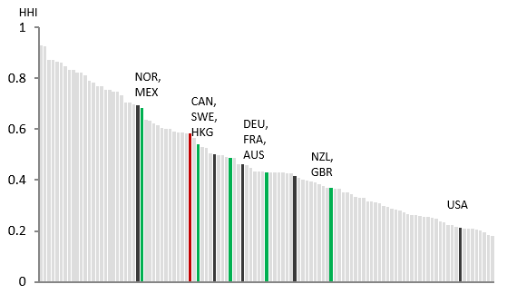
Text version
| Rank | HHI | ISO-3 code | Country |
|---|---|---|---|
| 1 | 0.928172 | MKD | Macedonia, FYR |
| 2 | 0.92625 | CPV | Cape Verde |
| 3 | 0.87278 | SER | Serbia, FR(Serbia/Montenegro) |
| 4 | 0.871491 | ALB | Albania |
| 5 | 0.863796 | MDA | Moldova |
| 6 | 0.862223 | BIH | Bosnia and Herzegovina |
| 7 | 0.845885 | SVK | Slovak Republic |
| 8 | 0.833282 | SVN | Slovenia |
| 9 | 0.83272 | KGZ | Kyrgyz Republic |
| 10 | 0.823744 | KWT | Kuwait |
| 11 | 0.82247 | CZE | Czech Republic |
| 12 | 0.811422 | POL | Poland |
| 13 | 0.791028 | HUN | Hungary |
| 14 | 0.782466 | LVA | Latvia |
| 15 | 0.769923 | LTU | Lithuania |
| 16 | 0.769271 | BLR | Belarus |
| 17 | 0.755607 | ROM | Romania |
| 18 | 0.755207 | BMU | Bermuda |
| 19 | 0.749098 | HRV | Croatia |
| 20 | 0.748593 | EST | Estonia |
| 21 | 0.734723 | LUX | Luxembourg |
| 22 | 0.705368 | ISL | Iceland |
| 23 | 0.705145 | BRN | Brunei |
| 24 | 0.69755 | NOR | Norway |
| 25 | 0.693027 | MEX | Mexico |
| 26 | 0.684681 | BGR | Bulgaria |
| 27 | 0.636988 | SLB | Solomon Islands |
| 28 | 0.633615 | WSM | Samoa |
| 29 | 0.623658 | MNT | Montenegro |
| 30 | 0.615113 | TUN | Tunisia |
| 31 | 0.603751 | BEL | Belgium |
| 32 | 0.601886 | KAZ | Kazakhstan |
| 33 | 0.6009 | MMR | Myanmar |
| 34 | 0.590167 | AZE | Azerbaijan |
| 35 | 0.587935 | NLD | Netherlands |
| 36 | 0.585672 | PRT | Portugal |
| 37 | 0.584762 | ARM | Armenia |
| 38 | 0.582959 | CAN | Canada |
| 39 | 0.565601 | GEO | Georgia |
| 40 | 0.539604 | SWE | Sweden |
| 41 | 0.530994 | TGO | Togo |
| 42 | 0.52731 | OMN | Oman |
| 43 | 0.506366 | FIN | Finland |
| 44 | 0.500991 | HKG | Hong Kong, China |
| 45 | 0.497159 | SGP | Singapore |
| 46 | 0.49666 | SUD | Sudan |
| 47 | 0.489503 | ESP | Spain |
| 48 | 0.487039 | DEU | Germany |
| 49 | 0.486817 | GRC | Greece |
| 50 | 0.463872 | ITA | Italy |
| 51 | 0.462144 | FRA | France |
| 52 | 0.458059 | DNK | Denmark |
| 53 | 0.446875 | UKR | Ukraine |
| 54 | 0.434189 | PHL | Philippines |
| 55 | 0.433743 | SLV | El Salvador |
| 56 | 0.433601 | MRT | Mauritania |
| 57 | 0.431625 | AUS | Australia |
| 58 | 0.431295 | NIC | Nicaragua |
| 59 | 0.430097 | DZA | Algeria |
| 60 | 0.429395 | DOM | Dominican Republic |
| 61 | 0.428461 | MLI | Mali |
| 62 | 0.427527 | MYS | Malaysia |
| 63 | 0.424989 | PLW | Palau |
| 64 | 0.417337 | NZL | New Zealand |
| 65 | 0.409947 | PRY | Paraguay |
| 66 | 0.402201 | NPL | Nepal |
| 67 | 0.396399 | IRL | Ireland |
| 68 | 0.393133 | TUR | Turkey |
| 69 | 0.389374 | BLZ | Belize |
| 70 | 0.3831 | JAM | Jamaica |
| 71 | 0.375143 | KOR | Korea, Rep. |
| 72 | 0.370104 | CMR | Cameroon |
| 73 | 0.368682 | GBR | United Kingdom |
| 74 | 0.364873 | ABW | Aruba |
| 75 | 0.36452 | FJI | Fiji |
| 76 | 0.352941 | IDN | Indonesia |
| 77 | 0.350903 | MUS | Mauritius |
| 78 | 0.345932 | RUS | Russian Federation |
| 79 | 0.334554 | NAM | Namibia |
| 80 | 0.331782 | CYP | Cyprus |
| 81 | 0.33112 | ZMB | Zambia |
| 82 | 0.316872 | JPN | Japan |
| 83 | 0.316506 | CHE | Switzerland |
| 84 | 0.313141 | UGA | Uganda |
| 85 | 0.308871 | HND | Honduras |
| 86 | 0.297866 | SEN | Senegal |
| 87 | 0.295606 | EGY | Egypt, Arab Rep. |
| 88 | 0.285967 | BOL | Bolivia |
| 89 | 0.28504 | CHL | Chile |
| 90 | 0.279403 | JOR | Jordan |
| 91 | 0.273456 | MDG | Madagascar |
| 92 | 0.264489 | COL | Colombia |
| 93 | 0.263332 | COG | Congo, Rep. |
| 94 | 0.262932 | MOZ | Mozambique |
| 95 | 0.259293 | ISR | Israel |
| 96 | 0.255781 | BDI | Burundi |
| 97 | 0.254558 | TZA | Tanzania |
| 98 | 0.251617 | ECU | Ecuador |
| 99 | 0.24764 | PER | Peru |
| 100 | 0.237767 | CHN | China |
| 101 | 0.235207 | LKA | Sri Lanka |
| 102 | 0.224822 | NGA | Nigeria |
| 103 | 0.223927 | PAK | Pakistan |
| 104 | 0.214931 | KEN | Kenya |
| 105 | 0.211206 | USA | United States |
| 106 | 0.208735 | GHA | Ghana |
| 107 | 0.208528 | URY | Uruguay |
| 108 | 0.207423 | BRA | Brazil |
| 109 | 0.204602 | BWA | Botswana |
| 110 | 0.201463 | ARG | Argentina |
| 111 | 0.194651 | ZAF | South Africa |
| 112 | 0.182994 | EUN | European Union |
| 113 | 0.17943 | IND | India |
5. Diversification outside of the United States
It is no surprise that Canada’s export patterns are largely dependent on the United States. The U.S. represents such a large proportion of Canada’s exports that trying to examine other countries is ineffective if the United States remains in the sample. Thus, to examine other countries, the United States needs to be excluded from the analysis.
Figure 4: Canada's Non-U.S. Export Shares
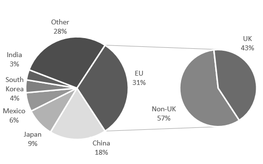
Text version
| Economy | Share | |
|---|---|---|
| EU | 0.315159 | |
| China | 18% | |
| Japan | 9% | |
| Mexico | 6% | |
| South Korea | 4% | |
| India | 3% | |
| Other | 28% | |
| Non-UK | 18% | 57.5% |
| UK | 13% | 42.5% |
Excluding the United States, Canada’s exports by country become much more diverse, with an HHI of 0.07 in 2017. Being diverse by non-U.S. country does not imply that Canada is immune to shocks from other countries; it implies that Canada’s economy should be able to adjust in the advent of a (non-U.S.) country-specific downturn. As Canadian exports are not dependent on any country outside of the United States, it reduces the impact of trade protectionist measures and gives Canada a more favourable bargaining position in trade negotiations. However, there could be potential benefits from further diversifying Canadian exports.
India, for example, makes up 0.8% of Canada’s exports, but its share of global GDP is 3.2%..Footnote 10, Footnote 11 The World Bank forecasts that India will be the 3rd fastest growing economy in the world between 2018 and 2020 (behind Ethiopia and Guyana). If Canadian firms are able to overcome the obstacles of exporting to a distant country, they stand to benefit from a high demand for Canadian products from one of the fastest growing markets.
6. Diversification within the United States
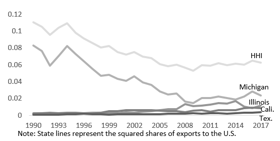
Previous arguments based on the gravity model were made to explain the high share of exports going to the United States. As was seen when aggregating countries into regions, Canada’s export patterns were reasonably normal. This analysis should also work the other way when the United States is disaggregated at the state level. The HHI of Canadian exports by U.S. state was 0.06 in 2017, indicating that exports are diverse at the state level.
Figure 5: HHI by U.S. State
Text version
| Year | HHI | Michigan | Illinois | California | Texas |
|---|---|---|---|---|---|
| 1990 | 0.110174 | 0.083069 | 0.002499 | 0.002027 | 0.000647 |
| 1991 | 0.104823 | 0.076438 | 0.00263 | 0.002681 | 0.000851 |
| 1992 | 0.095525 | 0.05912 | 0.002999 | 0.002306 | 0.000806 |
| 1993 | 0.103794 | 0.070491 | 0.002734 | 0.002255 | 0.000948 |
| 1994 | 0.109329 | 0.082384 | 0.003001 | 0.002487 | 0.001159 |
| 1995 | 0.097954 | 0.072865 | 0.003344 | 0.00232 | 0.001443 |
| 1996 | 0.090931 | 0.064025 | 0.002629 | 0.001974 | 0.0017 |
| 1997 | 0.085622 | 0.055344 | 0.003312 | 0.002117 | 0.001601 |
| 1998 | 0.080602 | 0.046937 | 0.002821 | 0.003336 | 0.001216 |
| 1999 | 0.081966 | 0.048002 | 0.002491 | 0.004658 | 0.001008 |
| 2000 | 0.075337 | 0.04302 | 0.002772 | 0.005095 | 0.00127 |
| 2001 | 0.071948 | 0.040737 | 0.003636 | 0.006264 | 0.001347 |
| 2002 | 0.075233 | 0.046509 | 0.003268 | 0.005816 | 0.001397 |
| 2003 | 0.069502 | 0.039031 | 0.004495 | 0.005916 | 0.001379 |
| 2004 | 0.068042 | 0.0359 | 0.005028 | 0.00623 | 0.001267 |
| 2005 | 0.060783 | 0.028449 | 0.006071 | 0.005338 | 0.001274 |
| 2006 | 0.058415 | 0.02473 | 0.007115 | 0.005163 | 0.001631 |
| 2007 | 0.059781 | 0.025972 | 0.00738 | 0.005016 | 0.002068 |
| 2008 | 0.056256 | 0.016468 | 0.013087 | 0.00394 | 0.001727 |
| 2009 | 0.052697 | 0.01443 | 0.010833 | 0.005736 | 0.002266 |
| 2010 | 0.059351 | 0.020446 | 0.011533 | 0.006215 | 0.002123 |
| 2011 | 0.05874 | 0.020742 | 0.012621 | 0.004198 | 0.002317 |
| 2012 | 0.061856 | 0.022224 | 0.014375 | 0.006319 | 0.00256 |
| 2013 | 0.059635 | 0.020582 | 0.014121 | 0.006268 | 0.001939 |
| 2014 | 0.061058 | 0.018971 | 0.016717 | 0.006246 | 0.002564 |
| 2015 | 0.060212 | 0.022548 | 0.010129 | 0.008526 | 0.002937 |
| 2016 | 0.064658 | 0.028141 | 0.008451 | 0.009382 | 0.003032 |
| 2017 | 0.062692 | 0.023698 | 0.011578 | 0.008802 | 0.003799 |
Goldfarb (2006) makes the argument that Canada already captures the benefits from diversification as it is diverse by U.S. region. Goldfarb’s argument drew from portfolio theory in finance, noting that the covariance of Canadian exports across U.S. regions lowered the volatility more than by diversifying across other major trading partners.Footnote 12 Although the analogy to a financial portfolio is not perfect, it conveys the message that diversification is a means to reduce export volatility and thus the focus does not necessarily have to be at a country level.Footnote 13 However, one of the premises of the paper was that a trade war with the United States was less likely than with any other country because “it is counterproductive to start cross-border trade disputes when production is highly integrated cross-border.” This was not a faulty reasoning on the part of Goldfarb, but illustrative of how conditions have changed. While Canada may reap more traditional economic benefits from diversification by being diverse across the U.S. states, being diverse by state is less useful to counter policy shocks, and thus it would be prudent to further diversify Canadian exports in non-U.S. markets.
7. Services
This study focuses primarily on merchandise trade due to data constraints for services, but Canada’s services trade is also important.Footnote 14 Since 1990, services exports have grown at an annual rate of 6.3%, while merchandise exports have grown at a rate of 4.9% per year. In 2017, services exports were larger than Canada’s energy exports ($114B vs. $110B), with the United States accounting for 55.8% of total services exports.Footnote 15 Although the United States still dominates Canada’s services trade, the share of services trade going to the U.S. is 20 percentage points lower than its share of Canada’s merchandise exports. Many of the arguments put forth in this paper support the view that Canada’s exports are more diverse than generally assumed, but this section will argue conversely that services trade is less diverse than generally assumed, and that the difference between services exports and merchandise exports is small.
Not all services exports should be treated equally in terms of trade diversification. Travel accounts for 23.1% of services trade, and transportation and government services for 16.3%. Travel should be excluded from the analysis; although it is important to the Canadian economy, the choice of foreigners traveling to Canada is not generally considered to be linked to trade policy.Footnote 16 Government services exports are likewise somewhat not pertinent to trade policy. Transportation services should also be excluded as they largely have to do with existing trade or travel—they are a necessary means to export, but not what firms export in and of itself.
Thus, the focus of export diversification should be on commercial services. In 2017, commercial services exports totaled $69 billion. Canada’s top partners in commercial services are the United States (64.9%), the United Kingdom (5.8%), France (2.4%), and Bermuda (2.4%).
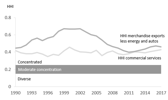
The hypothesis around services exports is generally that they are more diverse than merchandise trade exports (often, the 20 p.p. difference mentioned above is presented as evidence) because distance is not as important due to improving technology that allows instant communication anywhere in the world, enabling many services to be provided at great distance with little effort. To some extent this is true; while commercial services are less diverse than overall services exports, they are more diverse than merchandise exports. However, if energy and autos are excluded from merchandise trade, the gap between services and merchandise exports becomes small, especially since 2011.Footnote 17 The HHI for commercial services trade in 2017 was 0.43, compared to 0.46 for merchandise trade excluding energy and autos.Footnote 18 Unlike merchandise trade which saw a large change in export concentration over the sample period, services exports have stayed at a more consistent level. While commercial services exports are still more diverse than merchandise exports, the difference between the two is not as large as commonly believed.
Figure 6: Comparing the two HHI's
Text version
| Year | Commercial services HHI | HHI merchandise exports less energy and autos | Concentrated | Unconcentrated |
|---|---|---|---|---|
| 1990 | 0.41775 | 0.448118 | 0.25 | 0.15 |
| 1991 | 0.393539 | 0.453651 | 0.25 | 0.15 |
| 1992 | 0.381169 | 0.482877 | 0.25 | 0.15 |
| 1993 | 0.382046 | 0.540864 | 0.25 | 0.15 |
| 1994 | 0.394303 | 0.561384 | 0.25 | 0.15 |
| 1995 | 0.376734 | 0.533896 | 0.25 | 0.15 |
| 1996 | 0.350337 | 0.563616 | 0.25 | 0.15 |
| 1997 | 0.372343 | 0.581029 | 0.25 | 0.15 |
| 1998 | 0.363277 | 0.643197 | 0.25 | 0.15 |
| 1999 | 0.413617 | 0.670715 | 0.25 | 0.15 |
| 2000 | 0.456321 | 0.668155 | 0.25 | 0.15 |
| 2001 | 0.425597 | 0.669101 | 0.25 | 0.15 |
| 2002 | 0.403536 | 0.672827 | 0.25 | 0.15 |
| 2003 | 0.399176 | 0.633435 | 0.25 | 0.15 |
| 2004 | 0.392873 | 0.603015 | 0.25 | 0.15 |
| 2005 | 0.421247 | 0.58607 | 0.25 | 0.15 |
| 2006 | 0.359964 | 0.541713 | 0.25 | 0.15 |
| 2007 | 0.394014 | 0.489112 | 0.25 | 0.15 |
| 2008 | 0.413844 | 0.463237 | 0.25 | 0.15 |
| 2009 | 0.380131 | 0.44487 | 0.25 | 0.15 |
| 2010 | 0.371195 | 0.419307 | 0.25 | 0.15 |
| 2011 | 0.379702 | 0.399599 | 0.25 | 0.15 |
| 2012 | 0.401896 | 0.405404 | 0.25 | 0.15 |
| 2013 | 0.400118 | 0.419527 | 0.25 | 0.15 |
| 2014 | 0.392691 | 0.434979 | 0.25 | 0.15 |
| 2015 | 0.407543 | 0.461584 | 0.25 | 0.15 |
| 2016 | 0.418926 | 0.473342 | 0.25 | 0.15 |
| 2017 | 0.42786 | 0.460144 | 0.25 | 0.15 |
| Year | Theil | Gini | HHI | Normalized HHI | |
|---|---|---|---|---|---|
| 1990 | 3.827271 | 0.961108 | 0.565467 | 0.563131 | 0.611081 |
| 1991 | 3.799553 | 0.960436 | 0.568624 | 0.566227 | 0.604357 |
| 1992 | 3.906853 | 0.963442 | 0.599224 | 0.597033 | 0.634423 |
| 1993 | 4.151926 | 0.969759 | 0.648528 | 0.646779 | 0.697588 |
| 1994 | 4.174467 | 0.971328 | 0.662447 | 0.660725 | 0.71328 |
| 1995 | 4.148835 | 0.970739 | 0.630704 | 0.628954 | 0.707389 |
| 1996 | 4.212475 | 0.971106 | 0.657282 | 0.65565 | 0.711059 |
| 1997 | 4.231082 | 0.969982 | 0.671646 | 0.670067 | 0.699816 |
| 1998 | 4.370291 | 0.973541 | 0.719859 | 0.718506 | 0.735409 |
| 1999 | 4.492444 | 0.977105 | 0.752418 | 0.751239 | 0.771055 |
| 2000 | 4.540709 | 0.979063 | 0.757064 | 0.75594 | 0.790627 |
| 2001 | 4.55195 | 0.979126 | 0.758716 | 0.757609 | 0.791264 |
| 2002 | 4.535362 | 0.978504 | 0.760108 | 0.758987 | 0.785037 |
| 2003 | 4.459502 | 0.976186 | 0.736231 | 0.734998 | 0.761863 |
| 2004 | 4.390996 | 0.974332 | 0.714423 | 0.713089 | 0.743321 |
| 2005 | 4.357026 | 0.9728 | 0.703988 | 0.702611 | 0.727999 |
| 2006 | 4.252636 | 0.970008 | 0.666918 | 0.665391 | 0.700081 |
| 2007 | 4.106578 | 0.965544 | 0.625925 | 0.624186 | 0.655436 |
| 2008 | 4.035602 | 0.96199 | 0.60554 | 0.603722 | 0.619905 |
| 2009 | 3.927004 | 0.959339 | 0.567071 | 0.565075 | 0.593391 |
| 2010 | 3.934581 | 0.961016 | 0.564718 | 0.562693 | 0.610157 |
| 2011 | 3.888191 | 0.961293 | 0.546975 | 0.544858 | 0.612927 |
| 2012 | 3.94563 | 0.962705 | 0.560025 | 0.557988 | 0.627051 |
| 2013 | 3.986746 | 0.963817 | 0.57911 | 0.577143 | 0.638167 |
| 2014 | 4.048296 | 0.964906 | 0.593531 | 0.591692 | 0.649056 |
| 2015 | 4.024736 | 0.964065 | 0.592346 | 0.590458 | 0.640651 |
| 2016 | 4.032711 | 0.965401 | 0.585725 | 0.583834 | 0.654009 |
| 2017 | 4.024038 | 0.965146 | 0.579499 | 0.577596 | 0.651463 |
Further diversification of commercial services trade may prove difficult as it raises different challenges than merchandise trade. Services trade is heterogeneous across industries that have different regulations. (Meehan, 2014) In merchandise trade, a free-trade agreement would typically open up the whole market to most goods, but in services trade, the movement of people as well as the nuances of each service make this more difficult. Canada and the EU are currently working on a deal for the mutual recognition of professional designations which would certainly help diversify Canada’s commercial services.Footnote 19 However, to provide some scope of the difficulties surrounding this process, Canadian provinces do not always have mutual recognition of qualifications from other provinces, let alone other countries.
8. Conclusion
Canada’s merchandise exports are among the most concentrated in the world. This is entirely due to the high share going to the United States. However, from the perspective of regions, Canadian merchandise exports do not stand out, implying that Canada’s trade patterns actually are comparatively normal—this will make diversification more challenging as Canada’s exports will have to overcome natural economic forces. Canada’s merchandise exports are diverse by non-U.S. country and by U.S. state. Commercial services are marginally more diverse than merchandise exports, but not as diverse as is generally thought.
9. References
Beaulieu, Eugene, and Yang Song. "What Dependency Issues? Re-Examining Assumptions About Canada’s Reliance on the US Export Market." SPP Research Paper 8, no. 3 (January 29, 2015).
Brown, W. Mark. "How much thicker is the Canada–US border? The cost of crossing the border by truck in the pre-and post-9/11 eras." Research in transportation business & management 16 (2015): 50-66.
World Bank. Global Economic Prospects: Broad-Based Upturn, but for How Long? Washington, DC (January 2018), doi:10.1596/978-1-4648-1163-0. License: Creative Commons Attribution CC BY 3.0 IGO.
Goldfarb, D. (2006). "Too many eggs in one basket? Evaluating Canada's need to diversify trade" (Commentary). Retrieved December 05, 2018, from C.D. Howe Institute website: https://www.cdhowe.org/sites/default/files/attachments/research_papers/mixed/commentary_236.pdf.
Government of Canada, Trade Data Online, Retrieved from https://www.ic.gc.ca/app/scr/tdst/tdo/crtr.html?&productType=HS6&lang=eng.
Meehan, Lisa. "New Zealand's international trade in services: A background note." New Zealand Productivity Commission, 2014.
Statistics Canada. Table 36-10-0007-01: International transactions in services, by selected countries, annual (x 1,000,000).
Sydor, Aaron, and David Boileau (2006). China as a Link in Global Value Chains (2nd ed., Vol. 9, Horizons, pp. 49-55) (Government of Canada, Public Works and Government Services Canada) Ottawa, ON: Policy Research Initiative.
United Nations Statistics Division. UN Comtrade. New York: United Nations. Retrieved from: https://comtrade.un.org/data/.
WCS Source: Alberta Energy (Jan 2009 to present). Retrieved from: https://economicdashboard.alberta.ca/OilPrice.
World Bank, National Accounts data, and OECD, National Accounts data files. Retrieved from https://data.worldbank.org/indicator.
10. Appendix: Review of possible trade diversification measures
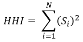
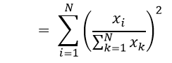
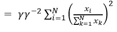
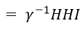
Herfindahl-Hirschman Index (HHI)
Text version
HHI at time t equals the sum from i equals one to N of the share of export i at time t squared.
; where Si denotes category i’s share of total exports (or trade) at time t.
This index constructs a score from zero to one. The closer the index is to one, the more concentrated is Canada’s trade. E.g. If Canada only traded with one country, the share of exports heading to the country would be 1 and the index would equal 1. Alternatively, if Canada’s trade was divided evenly between 100 different countries, the index would equal 0.01.
The HHI is the most common measure of trade concentration and is used to measure market concentration of potential mergers in anti-trust cases. The HHI has been used to study Canada’s export concentration by Global Affairs Canada’s Office of the Chief Economist, Statistics Canada, EDC, C.D. Howe, and the University of Calgary. Statistics Canada and the U.S. Department of Justice provide internationally accepted guidelines that a market is concentrated if the index is over 0.25, moderately concentrated if the index is between 0.15 and 0.25, and diverse if the index is below 0.15.
One drawback of the HHI is that it is sensitive to the level of aggregation. Because the shares are squared, the more disaggregated the data, the lower will be the level of the index. E.g. autos has a contribution of about 0.024 (0.1552) but splitting autos into cars and trucks (assuming a 50-50 split) would produce a combined contribution of only 0.012 (2[0.155/2]2).
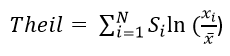
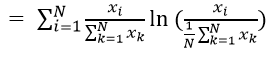
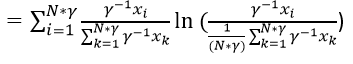
Theil Entropy Index
Text version
Theil Entropy Index at time t equals the sum from I equals one to N of the share of export i multiplied by the natural log of export i divided by the arithmetic mean of exports.
; where xi is the amount exported (traded) and µ is the arithmetic mean of the xi’s.
This index provides a value that is not bound by zero and one; a higher value indicates a higher degree of concentration. The index does not come with guidelines like the HHI, thus the only way to determine concentration from the index is to make comparisons either with other countries or over time with itself. The main advantage of the Theil index is that it has an exact decomposition to measure the effects of the extensive vs. intensive margin (i.e. trade becoming more diverse because Canada has gained new trade markets vs. diversifying by increasing trade in existing trade markets that previously had a small share). This decomposition can be very useful for small developing countries that are not in every market. However, Canada is already in essentially every market (product and geographic), so the decomposition may be less useful for Canada.
Additionally, the U.S. government recently switched to the Törnqvist-Theil price index for inflation adjustments (C-CPI-U), giving the index some clout. The main drawbacks of the index are that it is also sensitive to the level of aggregation and the formula is not as easy to understand as the HHI; furthermore, it is possible to describe the HHI by the “sum of squared shares”, but it is much harder to describe the Theil index without a mathematical formula.
The Gini Index
Text version
The Gini index at time tequals the double sum of I equals one to N and j equals one to N of the absolute value of the difference between export i and export j. This is the value of the numerator and is then divided by 2 multiplied by N multiplied by the sum from k equals one to N of export k.
The index is bound by zero and one, the closer to one, the more concentrated. Again, the index does not come with guidelines so making comparisons is the only way to assess concentration. The Gini index (or Gini coefficient) is often the main metric used in the income inequality literature. It is constructed by comparing the size of an individual export destination (product) with all other destinations (products). However, the main issue with the Gini index is that if one value is substantially bigger than the rest (e.g. the amount of exports Canada sends to the United States) the index will tend to be very close to one and have little variation.
Normalized HHI
Text version
The normalized HHI at time t equals the sum from i equals one to N of share of export i squared minus one which over N which is the numerator divided by one minus one over N.
This index takes the original HHI and adjusts it for category size. E.g. If there were three options, the lowest the regular HHI could be is 1/3rd, whereas if there are 100 options the lowest the index could be is 0.01. With the normalized HHI, the lowest the index can be is 0 in both cases. Canadian exports do not normally have a small sample size problem, and consequently the difference between the regular HHI and the normalized HHI would be small.
Finger-Kreinin Index
Text version
The Finger-Kreinin index for country j equals one half of the sum from i equals one to N of the absolute value of the difference between the share of export ij and export i
; where Sij is the share of commodity i in country j’s exports
Si is commodity i’s share of world exports.
This trade metric is a measure of relative export concentration, which indicates how one country’s export pattern differs from world exports. The United Nations Conference on Trade and Development (UNCTAD) publishes the index for a large number of countries and regions. This measure requires large amounts of data and is difficult to track over time as both the numerator (Canada) and the denominator (world) could change. Due to the need for data from other countries, the measure is more difficult to construct than others. Additionally, it is not clear that this measure would be useful for analyzing specifically Canada’s trade diversity.
Comparing the measures
Except for the Finger-Kreinin index, it is relatively easy to construct all the other measures for purposes of comparison. As previously mentioned, in the presence of a dominant share, the Gini index will tend to be close to 1 and show little variation. The index still shows the same pattern as the others, but the difference is in-between 0.96 and 0.98, which is difficult to show graphically. In order to make the Gini index more comparable, an affine transformation was performed by multiplying the index by 10 and subtracting 9. As can be seen from the figure, the indices all tell the same story about export diversification by country. It follows the negative parabola shape and is at approximately the same level now as it was in 1990. This is positive because it means that the analysis of trade diversification is insensitive to the measure chosen.
Figure 7: Export diversification by country
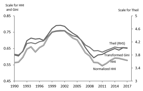
Text version
| Year | Theil | Gini | HHI | Normalized HHI | |
| 1990 | 3.827271 | 0.961108 | 0.565467 | 0.563131 | 0.611081 |
| 1991 | 3.799553 | 0.960436 | 0.568624 | 0.566227 | 0.604357 |
| 1992 | 3.906853 | 0.963442 | 0.599224 | 0.597033 | 0.634423 |
| 1993 | 4.151926 | 0.969759 | 0.648528 | 0.646779 | 0.697588 |
| 1994 | 4.174467 | 0.971328 | 0.662447 | 0.660725 | 0.71328 |
| 1995 | 4.148835 | 0.970739 | 0.630704 | 0.628954 | 0.707389 |
| 1996 | 4.212475 | 0.971106 | 0.657282 | 0.65565 | 0.711059 |
| 1997 | 4.231082 | 0.969982 | 0.671646 | 0.670067 | 0.699816 |
| 1998 | 4.370291 | 0.973541 | 0.719859 | 0.718506 | 0.735409 |
| 1999 | 4.492444 | 0.977105 | 0.752418 | 0.751239 | 0.771055 |
| 2000 | 4.540709 | 0.979063 | 0.757064 | 0.75594 | 0.790627 |
| 2001 | 4.55195 | 0.979126 | 0.758716 | 0.757609 | 0.791264 |
| 2002 | 4.535362 | 0.978504 | 0.760108 | 0.758987 | 0.785037 |
| 2003 | 4.459502 | 0.976186 | 0.736231 | 0.734998 | 0.761863 |
| 2004 | 4.390996 | 0.974332 | 0.714423 | 0.713089 | 0.743321 |
| 2005 | 4.357026 | 0.9728 | 0.703988 | 0.702611 | 0.727999 |
| 2006 | 4.252636 | 0.970008 | 0.666918 | 0.665391 | 0.700081 |
| 2007 | 4.106578 | 0.965544 | 0.625925 | 0.624186 | 0.655436 |
| 2008 | 4.035602 | 0.96199 | 0.60554 | 0.603722 | 0.619905 |
| 2009 | 3.927004 | 0.959339 | 0.567071 | 0.565075 | 0.593391 |
| 2010 | 3.934581 | 0.961016 | 0.564718 | 0.562693 | 0.610157 |
| 2011 | 3.888191 | 0.961293 | 0.546975 | 0.544858 | 0.612927 |
| 2012 | 3.94563 | 0.962705 | 0.560025 | 0.557988 | 0.627051 |
| 2013 | 3.986746 | 0.963817 | 0.57911 | 0.577143 | 0.638167 |
| 2014 | 4.048296 | 0.964906 | 0.593531 | 0.591692 | 0.649056 |
| 2015 | 4.024736 | 0.964065 | 0.592346 | 0.590458 | 0.640651 |
| 2016 | 4.032711 | 0.965401 | 0.585725 | 0.583834 | 0.654009 |
| 2017 | 4.024038 | 0.965146 | 0.579499 | 0.577596 | 0.651463 |
Sensitivity to data aggregation
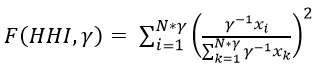
Both the HHI and Theil index are sensitive to the level of aggregation, thus a further criteria for selecting a measure could be how it responds to different levels of data aggregation. As long as the concentration is assessed using a consistent level of data, as was done in this analysis, the measure should not matter. But if comparisons are wanted at different levels of aggregation, the indices behave differently. The more disaggregated the data, the higher the Theil index becomes and the lower the HHI becomes. This is where guidelines become an issue with the HHI: do the guidelines of 0.15 and 0.25 correspond to the HS2 or HS4 data level?
The HHI is homogenous of order -1 when it comes to the amount of categories. For example, if the amount of categories were to double, with each category being even, the HHI would be exactly half.
Text version
HHI equals the sum from i equals one to N of the share of export i squared.
Text version
Which equals the sum from i equals one to N – open parenthesis – export i divided by the sum from k equals one to N of export k – close parenthesis – squared
Then dividing the data into equal groups,
And then, dividing the data into equal groups:
Text version
The function of HHI and gamma where gamma is the number of divisions in the data equals the sum of I equals one to N multiplied by gamma of – open parenthesis – inverse of gamma multiplied by export i, which is the numerator of the parenthesis. This is divided by the sum of k equals 1 to N multiplied by gamma of the inverse of gamma multiplied by export k– close parenthesis – squared.
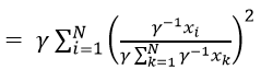
Where gamma is the number of divisions in the data,
Text version
The function of HHI and gamma then equals gamma multiplied by the sum of i equals one to N of – open parenthesis – inverse of gamma multiplied by export i divided by gamma multiplied by the sum of k equals one to N of inverse gamma multiplied by export k – close parenthesis – squared.
Since the summation is over the same N items; the summation of the first item to the Nth multiplied by gamma item is the same as gamma multiplied by the summation of the first to the Nth item.
Since the summation is over the same N items; the summation of the first item to the Nth multiplied by gamma item is the same as gamma multiplied by the summation of the first to the Nth item.
Text version
The function then equals gamma divided by gamma squared multiplied by the sum of I equals one to N of – open parenthesis – export i divided by the sum of k equals one to N of export k– close parenthesis – squared.
Text version
Which equals gamma inverse multiplied by the original HHI
Whereas the Theil index is homogenous of degree zero in product groups:
Whereas the Theil index is homogenous of degree zero in product groups:
Text version
The function then equals the sum of I equals 1 to N of export i divided by the denominator of the sum of k equals 1 to N of export k. This is then multiplied by the natural log of – open parenthesis – export i divided by the denominator of one over N multiplied by the sum of k equals 1 to N of export k– close parenthesis.
Then dividing the data, we get:
Text version
The Theil index equals the sum of i equals 1 to N multiplied by gamma of gamma inverse multiplied by export i divided by the sum of k equals 1 to N multiplied by gamma inverse multiplied by export k. This is multiplied by the natural log of – open parenthesis - the inverse of gamma multiplied by export i divided by the denominator which is one over N multiplied by gamma multiplied by the sum of k equals 1 to N multiplied by gamma of the inverse of gamma multiplied by export k – close parenthesis.
And then dividing the data:
Text version
The Theil index equals the sum of i equals 1 to N multiplied by gamma of gamma inverse multiplied by export i divided by the sum of k equals 1 to N multiplied by gamma inverse multiplied by export k. This is multiplied by the natural log of – open parenthesis - the inverse of gamma multiplied by export i divided by the denominator which is one over N multiplied by gamma multiplied by the sum of k equals 1 to N multiplied by gamma of the inverse of gamma multiplied by export k – close parenthesis.
Where gamma is the number of divisions in the data,
Text version
Which is equal to gamma multiplied by the sum of I equals 1 to N of the inverse of gamma multiplied by export i divided by the denominator which is gamma multiplied by the sum of k equals one to N of the inverse of gamma multiplied by export k. We then multiply this by the natural log of – open parenthesis – the inverse of gamma multiplied export i, divided by the denominator of – open bracket - gamma over N multiplied by gamma –close bracket – multiplied by the sum of k equals one to N of gamma inverse multiplied by export k – close parenthesis.
Text version
This then equals the inverse of gamma multiplied by gamma multiplied by the sum of I equals one to N of export i divided by the denominator of the sum of k equals 1 to N of export k. This is multiplied by the natural log of – open parenthesis – the inverse of gamma multiplied by export i, divided by the denominator which is the inverse of gamma over N multiplied by the sum of k equals one to N of export k– close parenthesis.
Text version
Which equals the sum of i equals one to N of export i divided by the sum of k equals one to N of export k. Multiplied by the natural log of – open parenthesis - the export i divided by the denominator of one over N times the sum of k equals one to N of export k – close parenthesis.

Text version
Which equals the Theil index.
However, it will never be the case that the disaggregation of trade data will be a division into equal parts. For example, hypothetically going from worldwide-level exports to country-level exports, each country does not receive an equal share of Canadian exports; one country (the United States) receives a much larger proportion than any other country. Thus, it is necessary to do the analysis by looking at non-even splits. For simplicity, the indices are split in two by giving one category a share of λ, and the other a share of 1-λ.
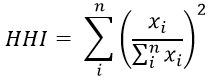
Text version
HHI equals the sum of I to N of – open parenthesis – export i traded divided by the sum of I to n of export i – close parenthesis – squared.
Then, splitting the data into two groups where 0 < λ < 1.
Then, splitting the data into two groups where 0 < λ < 1.
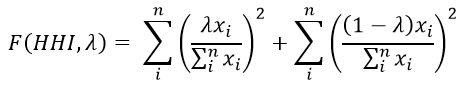
Text version
The function of HHI and lambda equals the sum of i to n of – open parenthesis –lambda multiplied by export i divided by the denominator which is the sum of I to n of export i – close parenthesis squared. Then add this to the sum of I to n of – open parenthesis - , - open bracket – one minus lambda– close bracket multiplied by export i divided by the denominator of the sum of I to n of export i – close parenthesis – squared.
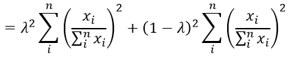
Text version
The function then equals lambda squared multiplied by the sum of i to n of – open parenthesis – export i divided by the sum of I to n export i – close parenthesis – squared plus – open bracket – one minus lambda – close bracket – squared multiplied by sum of I to n of – open parenthesis of export i divided by sum of I to n of export i– close parenthesis – squared.
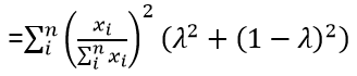
Text version
Then the sum of I to n of – open parenthesis – export i divided by sum of I to n of export i – close parenthesis – squared multiplied by - open parenthesis – lambda squared plus –open bracket – one minus lambda – close bracket – squared – close parenthesis.
Text version
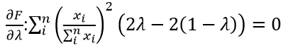
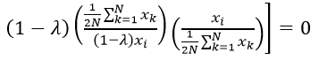
Taking the partial derivative with respect to lambda is the sum of I to n of – open parenthesis – export i divided by the sum of I to n of export i - close parenthesis – squared. We then multiply this by – open parenthesis – lambda multiplied by two minus two times – open bracket – one minus lambda – close bracket – close parenthesis - equals zero.

Text version
ambda star equals zero point five
Text version
The second order partial with respect to lambda equals the sum of I to n of – open parenthesis – export i divided by the sum of I to n of export i– close parenthesis – squared. This is multiplied by – open bracket – two plus two – close bracket. Which is greater than zero. For the Theil index:
Thus, the minimum value of the HHI is achieved at λ=0.5, but moreover the second derivative with respect to λ is positive, which implies that the function is decreasing until the minimum. This also implies that disaggregating the data will always decrease the HHI.
For the Theil index:
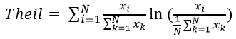
Text version
Theil index is equal to the sum of I equals 1 to N of - open parenthesis – export i divided by the sum of k equals 1 to N of export i – close parenthesis. Multiplied by the natural log of – open parenthesis – export i divided by – open bracket -one over N multiplied by the sum of k equals 1 to N of export k – close bracket – close parenthesis.
Splitting the data into two groups:
Splitting the data into two groups:

Text version
The function of Theil index and lambda equals the sum of i equals one to N of – open parenthesis – lambda multiplied by export i, divided by the sum of k equals one to N of export k – close parenthesis. We then multiply this by the natural log of – open parenthesis – lambda multiplied by export i, divided by –open bracket – one over two times N multiplied by the sum of k equals one to N of export k– close bracket – close parenthesis. We then add this to the sum of i equals one to N – open parenthesis – open bracket – one minus lambda – close bracket multiplied by export i. We then divide this by the denominator which is the sum of k equals one to N of export k – close parenthesis. We then multiply this by the natural log of – open parenthesis – open bracket – one minus lambda – close bracket - multiplied by export i, divided by – open bracket – one over two times N multiplied by the sum of k equals one to N of export k – close bracket – close parenthesis.
Text version
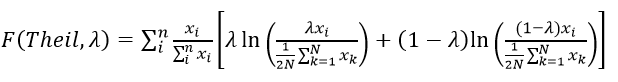
The function of Theil index and lambda equals the sum of i equals one to n of –open parenthesis - export i, divided by the sum of i equals one to n of export i – close parenthesis. We multiply this by – open big bracket – lambda multiplied by the natural log of – open parenthesis – lambda multiplied by export i, divided by – open bracket – one over two times N multiplied by the sum of k equals one to N of export k – close bracket – close parenthesis. We add this to – open bracket – one minus lambda – close bracket – multiplied by the natural log of – open parenthesis – open bracket – one minus lambda – close bracket - multiplied by export i, divided by – open bracket – one over two times N multiplied by the sum of k equals one to N of export k – close bracket – close parenthesis – close big bracket.

Text version
The derivative of the function with respect to lambda is the sum of i to n of - open parenthesis – the export i divided by the sum of I to n of export i – close parenthesis and we multiply this by – open big bracket – lambda multiplied by the natural log of – open parenthesis – lambda multiplied by export i, divided by – open bracket – one over two times N multiplied by the sum of k equals one to N of export k– close bracket – close parenthesis. We add this to lambda multiplied by – open parenthesis – one over two times N multiplied by the sum of k equals one to N of export k divided by lambda multiplied by export i– close parenthesis – multiplied by the– open parenthesis – export i divided by the denominator of bracket – one over two times N multiplied by the sum of k equals one to N of export k– close parenthesis. We then subtract the natural log of – open parenthesis – open bracket – one minus lambda – close bracket - multiplied by export i, divided by – open bracket – one over two times N multiplied by the sum of k equals one to N of export k – close bracket – close parenthesis. Finally we subtract – open bracket – one minus lambda – close bracket – multiplied by one over two times N multiplied by the sum of k equals one to N of export k, divided by the denominator – open bracket - one minus lambda – close bracket – multiplied by export i – close parenthesis – multiplied by – open parenthesis – export i divided by the denominator of bracket – one over two times N multiplied by the sum of k equals one to N of export k – close parenthesis – close big bracket – equals zero.
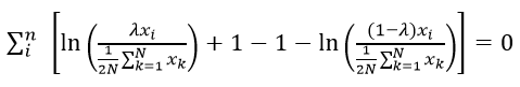
Text version
Now we have the sum of i to n of – open big bracket – the natural log of –open parenthesis – lambda multiplied by export i, divided by – open bracket – one over two times N multiplied by the sum of k equals one to N of export k – close bracket – close parenthesis plus one minus one minus the natural log of –open parenthesis – open bracket - one minus lambda – close bracket - multiplied by export i, divided by – open bracket – one over two times N multiplied by the sum of k equals one to N of export k– close parenthesis – close big bracket – equals zero.

Text version
lambda star equals one half
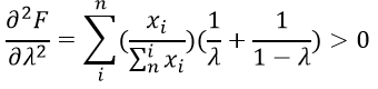
Text version
The second order partial with respect to lambda equals the sum of I to n of – open bracket – export i divided by the sum of n to I of export i – close bracket multiplied by – open bracket – one over lambda plus one divided by –open bracket - one minus lambda –close bracket – close bracket. Which is greater than zero.
Thus, the Theil index also reaches a minimum when the split is equal between two groups. However, from the previous result, the Theil index does not change when the split is even. Because the Theil index is concave with respect to λ it must increase whenever there is a non-even split of the data.
Deciding between the HHI and the Theil index depends on how one believes the division of the data should affect the concentration. If the view is that more categories means greater diversity, than the HHI would be better. Conversely, if the view is that disaggregating into anything other than an even split is further concentration, than the Theil index would be preferable.
- Date modified: